File:Circular convolution example.svg

Size of this PNG preview of this SVG file: 462 × 486 pixels. Other resolutions: 228 × 240 pixels | 456 × 480 pixels | 730 × 768 pixels | 973 × 1,024 pixels | 1,947 × 2,048 pixels.
Original file (SVG file, nominally 462 × 486 pixels, file size: 40 KB)
Captions
Captions
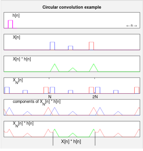
Example of using circular convolution to produce linear convolution
Summary edit
| Description |
English: Circular convolution can be expedited by the FFT algorithm, so it is often used with an FIR filter to efficiently compute linear convolutions. These graphs illustrate how that is possible. Note that a larger FFT size (N) would prevent the overlap that causes graph #6 to not quite match all of #3. |
|||
| Date | ||||
| Source | Own work | |||
| Author | Bob K | |||
| Permission (Reusing this file) |
I, the copyright holder of this work, hereby publish it under the following license:
|
|||
| Other versions |
This file was derived from: Circular convolution example.png |
|||
| SVG development | This W3C-invalid vector image was created with LibreOffice. |
|||
| Gnu Octave source | click to expand
This graphic was created with the help of the following Octave script: % Options
frame_background_gray = true;
if frame_background_gray
graphics_toolkit("qt") % has "insert text" option
% graphics_toolkit("fltk") % has cursor coordinate readout
frame_background = .94*[1 1 1];
d = 2; % amount to add to text sizes
else
graphics_toolkit("gnuplot") % background will be white regardless of value below
frame_background = .94*[1 1 1];
d=0;
endif
% (https://octave.org/doc/v4.2.1/Graphics-Object-Properties.html#Graphics-Object-Properties)
% Speed things up when using Gnuplot
set(0, "DefaultFigureColor",frame_background)
set(0, "DefaultAxesFontsize",10+d) % size of numeric tick labels
set(0, "DefaultTextFontsize",12+d)
set(0, "DefaultAxesXtick",[])
set(0, "DefaultAxesYtick",[])
set(0, "DefaultLineLinewidth",1)
xmax = 3000;
%=======================================================
hfig = figure("position",[100 100 488 512], "color",frame_background);
x1 = .02; % left margin
x2 = .02; % right margin
y1 = .08; % bottom margin for annotation
y2 = .08; % top margin for title
dy = .04; % vertical space between rows
width = 1-x1-x2;
height= (1-y1-y2-5*dy)/6; % space allocated for each of 6 rows
x_origin = x1;
y_origin = 1; % start at top of graph area
%=======================================================
y_origin = y_origin -y2 -height; % position of top row
% subplot() undoes all the "color" attempts above. (gnuplot bug)
subplot("position",[x_origin y_origin width height])
L = 100;
f = ones(1,L)/L;
plot(-100:200-1, [zeros(1,100) f*L zeros(1,100)], "linewidth",2, "color","magenta")
xlim([-100 xmax]); ylim([0 2])
title("Circular convolution example", "fontsize",16)
text(100, 1.6, "h[n]")
%text(xmax/2, 0.4, '\leftarrow n \rightarrow')
text(2500, 0.330, '\leftarrow n \rightarrow')
y_origin = y_origin -dy -height;
subplot("position",[x_origin y_origin width height])
a = [zeros(1,20) ones(1,L) zeros(1,300) 0.5*ones(1,100) zeros(1,1000-L-20-400)];
b = [zeros(1,1000-L-20) ones(1,L) zeros(1,20)];
a1 = [zeros(1,1000) a zeros(1,1000)];
b1 = [zeros(1,1000) b zeros(1,1000)];
plot(1:length(a1), a1, "color","blue", 1:length(a1), b1, "color","red")
xlim([0 xmax]); ylim([0 2])
text(200, 1.6, "X[n]")
y_origin = y_origin -dy -height;
subplot("position",[x_origin y_origin width height])
a1 = conv(a1,f);
b1 = conv(b1,f);
plot(1:length(a1), a1+b1, "color","green", "linewidth",2)
xlim([0 xmax]); ylim([0 2*max(a1)])
text(200, 1.6, "X[n] * h[n]")
%text(200, 1.6, "X[n] ∗ h[n]", "interpreter","none") % requires PERL post-processor
y_origin = y_origin -dy -height;
subplot("position",[x_origin y_origin width height])
a = [a a a];
b = [b b b];
L = 1:length(a);
plot(L, a, "color","blue", L, b, "color","red")
xlim([0 xmax]); ylim([0 2.5])
set(gca,"xtick", [1000 2000]);
%set(gca,"xticklabel",["N" "2N"])
set(gca,"xticklabel",[]); text(981,-.5, "N"); text(1955,-.5, "2N")
text(200, 2.0, 'X_N[n]')
y_origin = y_origin -dy -height;
subplot("position",[x_origin y_origin width height])
a1 = conv(a,f);
b1 = conv(b,f);
b1(1:90) = b1(3000+[1:90]);
L = 1:length(a1);
plot(L,a1,"color","blue", L,b1, "color","red")
xlim([0 xmax]); ylim([0 2*max(a1)])
text(200, 1.6, 'components of X_N[n] * h[n]') % can't use "interpreter","none" here
y_origin = y_origin -dy -height;
subplot("position",[x_origin y_origin width height])
c = a1+b1;
L = length(c);
k=1100;
plot(1:k, c(1:k), "color","red", k+(1:900), c(k+(1:900)), "color","green",...
"linewidth",2, (k+900+1):xmax, c((k+900+1):xmax), "color","red")
xlim([0 xmax]); ylim([0 2*max(a1+b1)])
text(200, 1.6, 'X_N[n] * h[n]') % can't use "interpreter","none" here
text(1263, -.6, "X[n] * h[n]", "fontsize",16)
%text(1274, -.6, "X[n] ∗ h[n]", "interpreter","none", "fontsize",16) % requires PERL post-processor
% After a call to annotation(), the cursor coordinates change to the units used below.
annotation("line", [.367 .367], [.113 .022])
annotation("line", [.664 .664], [.113 .022])
|
File history
Click on a date/time to view the file as it appeared at that time.
| Date/Time | Thumbnail | Dimensions | User | Comment | |
|---|---|---|---|---|---|
| current | 00:17, 29 January 2020 | | 462 × 486 (40 KB) | Bob K (talk | contribs) | replace white figure background with gray |
| 17:03, 9 June 2019 |  | 610 × 640 (130 KB) | Bob K (talk | contribs) | fixed script typo (bug) | |
| 14:47, 7 June 2019 |  | 610 × 640 (130 KB) | Bob K (talk | contribs) | reduce side margins | |
| 14:55, 5 June 2019 |  | 610 × 640 (135 KB) | Bob K (talk | contribs) | enlarge xlabel of subplot 1 | |
| 13:50, 5 June 2019 |  | 512 × 537 (332 KB) | Bob K (talk | contribs) | fix a problem with xlabel, caused by PERL post-processor (interferes with \leftarrow and \rightarrow) | |
| 13:29, 5 June 2019 |  | 512 × 537 (332 KB) | Bob K (talk | contribs) | Replace a couple of asterisks with ∗ (∗). But this requires the Octave output file to be post-processed by the PERL script that is also used for window function plots. | |
| 14:01, 4 June 2019 |  | 610 × 640 (135 KB) | Bob K (talk | contribs) | User created page with UploadWizard |
You cannot overwrite this file.
File usage on Commons
The following 9 pages use this file:
- User:Paris 16/Recent uploads/2019 June 4-6
- User:Paris 16/Recent uploads/2019 June 7-9
- User:Paris 16/Recent uploads/2020 January 29-31
- Commons:WikiProject Aviation/recent uploads/2019 June 4
- Commons:WikiProject Aviation/recent uploads/2019 June 5
- Commons:WikiProject Aviation/recent uploads/2019 June 7
- Commons:WikiProject Aviation/recent uploads/2019 June 9
- Commons:WikiProject Aviation/recent uploads/2020 January 29
- File:Circular convolution example.png
File usage on other wikis
The following other wikis use this file:
- Usage on en.wikipedia.org
- Usage on fr.wikipedia.org