File:Dandelion clock quarter dft dct.png
Original file (1,140 × 1,428 pixels, file size: 542 KB, MIME type: image/png)
Captions
Captions
Summary edit
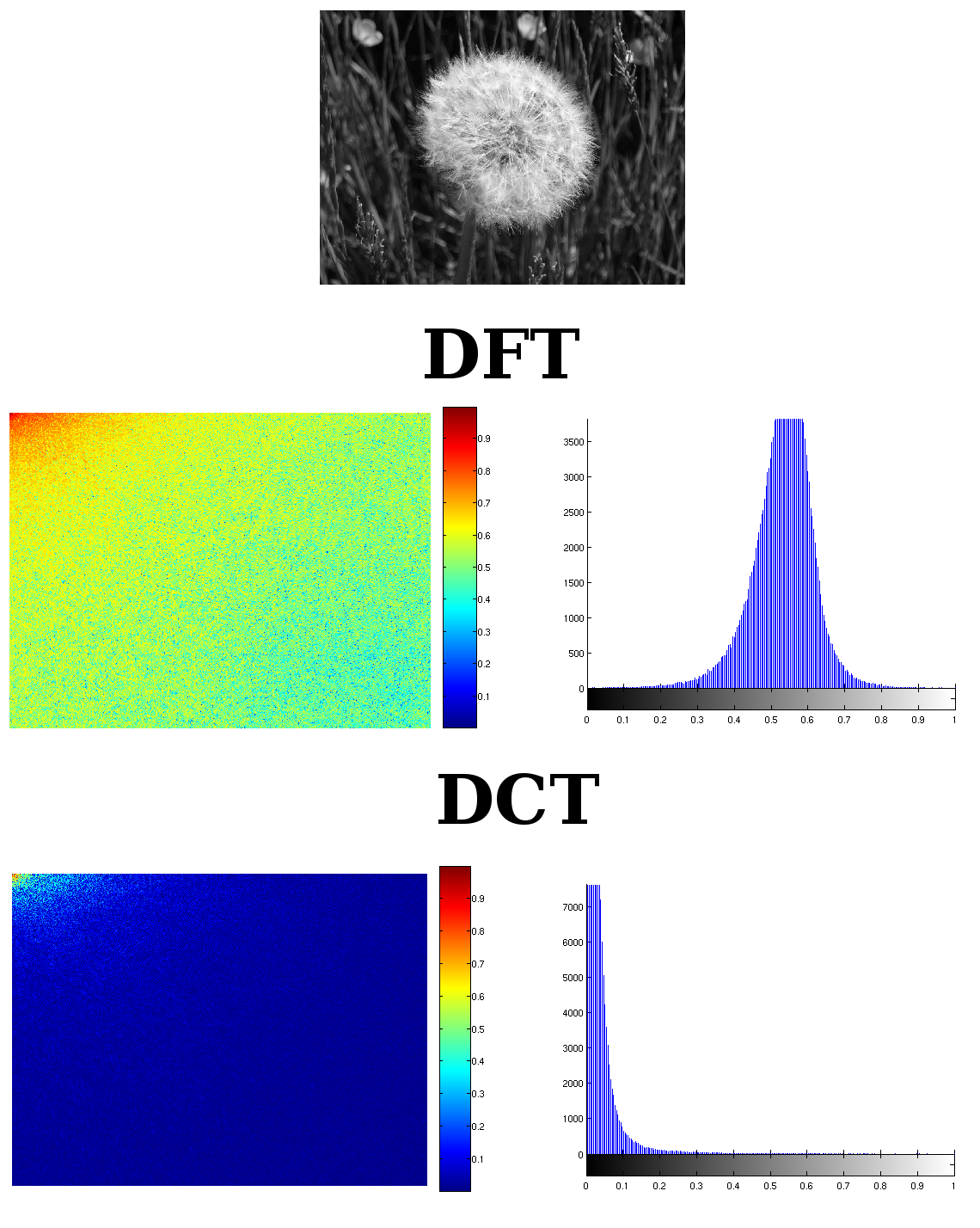
| Description | the picture shows the difference between the DFT and a DCT of an image |
| Date | |
| Source | I made it by myself |
| Author | Alessio Damato |
| Permission (Reusing this file) |
multilicensed (see below) |
| Other versions | the original image that was processed was Image:Dandelion_clock.jpg |
I used Image:Dandelion_clock.jpg to create this image. I wanted to show clearly the different behavior between the DFT and the DCT in the frequency domain.
The pictures are made of other figures. The first one on the top is just the original image: I used its gray-scale version. On the second line there is the DFT: its magnitude on the left, its histogram on the right. On the third line there is the DCT, with both magnitude and histogram.
The spectrum of the DFT has cropped so that the lowest frequencies are on the top-left of the picture, just like in the DCT. It is not such a rigorous process: the DFT in general is composed of two symmetric halves, but I put on the picture just one quarter, thus removing one quarter of necessary information. I did so to create an output that could be easily be compared with the DCT. Because of symmetry, I cropped to 1/4 the DCT as well, keeping the lower frequencies. Anyway it is clear how the DCT concentrates most of the energy into the lowest frequencies.
I created the single images with the following Matlab code:
% read the image
RGB = imread('Dandelion_clock.jpg');
% convert pixels to the [0 1] range
RGB = im2double(RGB);
% convert to grayscale
I = rgb2gray(RGB);

% calculate the size of the image and then divide
% by two, in order to crop it later
[X Y] = size(I);
Y = round(Y/2);
X = round(X/2);

% evaluate magnitude of the DFT
F = abs(fft2(I));
% take only a quarter
F = imcrop(F,[0 0 Y X]);
% use log scale
F = log(1 + F);
F = log(1 + F);
% normalize
F = F/max(F(:));

% evaluate magnitude of the DCT
C = abs(dct2(I));
% take only a quarter
C = imcrop(C,[0 0 Y X]);
% use log scale
C = log(1 + C);
C = log(1 + C);
% normalize
C = C/max(C(:));

% show all the results
imshow(F), colorbar, colormap(jet);
figure, imhist(F);
figure, imshow(C), colorbar, colormap(jet);
figure, imhist(C);
First it imports the RGB image and converts it to gray-scale. Then calculates the magnitude of both the transforms. Both pictures had a huge dynamic, so I calculated the logarithm of both, twice, in order to be able to show the transforms properly. Once all the pictures were shown on the screen, I just selected File -> Save as on Matlab to save all the pictures. I put them all together using Gimp.
(comment by RCL) I cant speak english very well, but I'm going to try it. The use of this code it's WRONG, we can't use this MATLAB code for comparing both transforms, because in MATLAB the definition of the DFT isn't normalized and the definition of the DCT in MATLB it's normalized. So we should multiply the result of the fft by a factor of 1.0/N², before we use the function abs. The result between the DFT and the DCT is very similar if we do this, but we can obtain the shannon entropy of the energy of both transforms and the result is that the entropy of the energy in the DCT is lower than the DFT, for that reason we say that the DCT compact the energy more than the DFT. I made my master thesis on the DCT.
Licensing edit

|
Permission is granted to copy, distribute and/or modify this document under the terms of the GNU Free Documentation License, Version 1.2 or any later version published by the Free Software Foundation; with no Invariant Sections, no Front-Cover Texts, and no Back-Cover Texts. A copy of the license is included in the section entitled GNU Free Documentation License. |
| This file is licensed under the Creative Commons Attribution-Share Alike 3.0 Unported license. | ||
| ||
| This licensing tag was added to this file as part of the GFDL licensing update. |
- You are free:
- to share – to copy, distribute and transmit the work
- to remix – to adapt the work
- Under the following conditions:
- attribution – You must give appropriate credit, provide a link to the license, and indicate if changes were made. You may do so in any reasonable manner, but not in any way that suggests the licensor endorses you or your use.
- share alike – If you remix, transform, or build upon the material, you must distribute your contributions under the same or compatible license as the original.
File history
Click on a date/time to view the file as it appeared at that time.
| Date/Time | Thumbnail | Dimensions | User | Comment | |
|---|---|---|---|---|---|
| current | 18:50, 13 May 2006 | | 1,140 × 1,428 (542 KB) | Alejo2083 (talk | contribs) | == Summary == {{Information| |Description= the picture shows the difference between the DFT and a DCT of an image |Source= I made it by myself |Date= 13/05/2006 |Author= Alessio Damato |Permission= multilicensed (see below) |other_versions= the original |
You cannot overwrite this file.
File usage on Commons
There are no pages that use this file.
File usage on other wikis
The following other wikis use this file:
- Usage on ar.wikipedia.org
- Usage on ca.wikipedia.org
- Usage on cs.wikipedia.org
- Usage on es.wikipedia.org
- Usage on eu.wikipedia.org
- Usage on it.wikipedia.org
- Usage on ja.wikipedia.org
- Usage on pt.wikipedia.org
- Usage on zh.wikipedia.org