File:Equipotential by Zureks.png

Size of this preview: 366 × 600 pixels. Other resolutions: 146 × 240 pixels | 639 × 1,047 pixels.
Original file (639 × 1,047 pixels, file size: 111 KB, MIME type: image/png)
Captions
Captions
Add a one-line explanation of what this file represents
Summary edit
| Description |
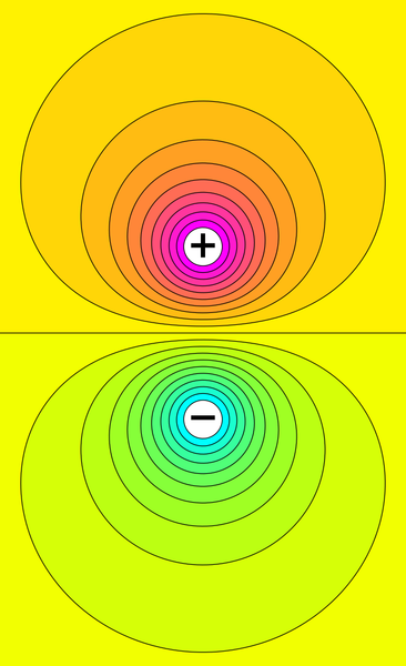
English: Voltage distribution between two electrically charged spheres (purple = positive voltage, blue = negative voltage). The black curves show equipotential contours. |
|||
| Date | ||||
| Source | Own work | |||
| Author | Zureks | |||
| Other versions |
|


Source code edit
The image can be created with Python Matplotlib using the following code:
import numpy as np
from matplotlib import pyplot as plt
from matplotlib import colors

cmap = colors.ListedColormap([np.clip((2*x, 2*(1-x), 4*(x-0.5)**2), 0, 1) for x in np.linspace(0., 1., 256)])

w, h = 639, 1047
xmax = 2.36
ymax = xmax * float(h) / float(w)
vmax = 0.78
y0 = 1.0
nlevels = 21
levels = np.linspace(-vmax, vmax, nlevels)
X, Y = np.mgrid[-xmax:xmax:250j, -ymax:ymax:800j]

# potential of two point charges
V  = 1.0 / np.maximum(np.sqrt(X**2 + (Y - y0)**2), 1e-2)
V -= 1.0 / np.maximum(np.sqrt(X**2 + (Y + y0)**2), 1e-2)

# rescale potential globally to make contour areas similar
V = (np.sqrt(1 + V * V) - 1) / V

plt.figure(figsize=(w/90., h/90.)).add_axes([0, 0, 1, 1])
contf = plt.contourf(X, Y, V, levels=levels, cmap=cmap,
         vmin=-vmax*(nlevels-1.)/nlevels, vmax=vmax*(nlevels-1.)/nlevels)
cont = plt.contour(X, Y, V, levels=contf.levels, colors='k', linestyles='solid')

plt.xticks([]), plt.yticks([])
plt.gca().set_aspect(aspect='equal')
plt.gca().axis('off')
plt.text(0, -y0, u'\u2212', size=48,fontweight='bold', ha='center', va='center')
plt.text(0, y0, '+', size=48,fontweight='bold', ha='center', va='center')
plt.savefig('Equipotential_of_dipole.png')
Licensing edit
| This file is made available under the Creative Commons CC0 1.0 Universal Public Domain Dedication. | |
| The person who associated a work with this deed has dedicated the work to the public domain by waiving all of their rights to the work worldwide under copyright law, including all related and neighboring rights, to the extent allowed by law. You can copy, modify, distribute and perform the work, even for commercial purposes, all without asking permission.
|
File history
Click on a date/time to view the file as it appeared at that time.
| Date/Time | Thumbnail | Dimensions | User | Comment | |
|---|---|---|---|---|---|
| current | 21:09, 16 May 2018 | | 639 × 1,047 (111 KB) | Geek3 (talk | contribs) | Replaced with analytically computed precise contour shapes. The old version which came from an FEM simulation had significant errors towards the edges, possibly because the simulation volume was chosen too small. The potential dropped much too slowly towards the image edges. In contrast, the analytic solution is very simple, as the potential is just the linear sum of two 1/r potentials. |
| 16:37, 11 April 2010 |  | 639 × 1,047 (32 KB) | Zureks (talk | contribs) | {{Information |Description={{en|1=Voltage distribution between two electrically charged spheres (purple = positive voltage, blue = negative voltage). The black curves show equipotential contours.}} |Source={{own}} |Author=Zureks |Date=2010 |
You cannot overwrite this file.
File usage on Commons
There are no pages that use this file.
File usage on other wikis
The following other wikis use this file:
- Usage on ar.wikipedia.org
- Usage on be-tarask.wikipedia.org
- Usage on cs.wikipedia.org
- Usage on cv.wikipedia.org
- Usage on fi.wikipedia.org
- Usage on fr.wikipedia.org
- Usage on ht.wikipedia.org
- Usage on kk.wikipedia.org
- Usage on ko.wikipedia.org
- Usage on no.wikipedia.org
- Usage on oc.wikipedia.org
- Usage on ru.wikipedia.org
- Usage on sl.wikipedia.org
- Usage on uk.wikipedia.org
- Usage on www.wikidata.org
- Usage on zh.wikipedia.org