File:Testsimulation der Vermögenskonzentration nach Fargione mit Vermögensteuern.png

Size of this preview: 800 × 267 pixels. Other resolutions: 320 × 107 pixels | 640 × 213 pixels.
Original file (1,800 × 600 pixels, file size: 110 KB, MIME type: image/png)
Captions
Captions
Add a one-line explanation of what this file represents
Summary
edit
| Description |
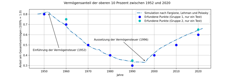
Deutsch: Nur ein Test, ob die Simulation für die Bundesrepublik Deutschland zu gebrauchen ist. |
| Date | |
| Source | Own work |
| Author | Majow |
| PNG development | This plot was created with Matplotlib. |
| Source code | Python code# Entrepreneurs, Chance, and the Deterministic Concentration of Wealth
# Joseph E. Fargione, Clarence Lehman, Stephen Polasky
# https://doi.org/10.1371/journal.pone.0020728
import numpy as np # Für Rechnungen mit Vektoren
import matplotlib.pyplot as plt # Für die Erstellung der Grafik
n, t1, t2, t3 = 10000, 80, 44, 26 # Populationsgröße und Zeiträume (Jahre)
mu, sigma, tax = 0.05, 0.25, 0.15 # Mittelwert, Streuung und Vermögensteuer
n_top, n_tax = 10, 10 # Betrachte die oberen 10% (Einer von 10)
top_n, tax_n = n // n_top, n // n_tax # Besteuere die oberen 10% (Einer von 10)
X = np.zeros(n) # Simulation beginnt mit Gleichverteilung
Y = np.exp(X) # Berechnung der Kapitalvermögen
W = Y[0:n].sum() # Berechnung des Gesamtvermögens
Q = np.zeros(t1+t2+t3+1) # Speicherplatz für die Vermögensanteile
Q[0] = Y[n-top_n:n].sum() / W # Vermögensanteil speichern (Quotient)
# Erste Simulation (ohne Steuern)
for i in range(t1):
R = np.random.normal(mu, sigma, n) # Ziehung der zufälligen Raten
X = X + R # Berechnung der Exponenten
X.sort() # Sortierung der Exponenten
Y = np.exp(X) # Berechnung der Kapitalvermögen
W = Y[0:n].sum() # Berechnung des Gesamtvermögens
Q[i+1] = Y[n-top_n:n].sum() / W # Vermögensanteil speichern (Quotient)
# Zweite Simulation (mit Steuern)
for i in range(t2):
X[n-tax_n:n] = X[n-tax_n:n] - tax # Abzug der Steuern an der Spitze
R = np.random.normal(mu, sigma, n) # Ziehung der zufälligen Raten
X = X + R # Berechnung der Exponenten
X.sort() # Sortierung der Exponenten
Y = np.exp(X) # Berechnung der Kapitalvermögen
W = Y[0:n].sum() # Berechnung des Gesamtvermögens
Q[t1+i+1] = Y[n-top_n:n].sum() / W # Vermögensanteil speichern (Quotient)
# Dritte Simulation (ohne Steuern)
for i in range(t3):
R = np.random.normal(mu, sigma, n) # Ziehung der zufälligen Raten
X = X + R # Berechnung der Exponenten
X.sort() # Sortierung der Exponenten
Y = np.exp(X) # Berechnung der Kapitalvermögen
W = Y[0:n].sum() # Berechnung des Gesamtvermögens
Q[t1+t2+i+1] = Y[n-top_n:n].sum() / W # Vermögensanteil speichern (Quotient)
fig, ax = plt.subplots(figsize=(12, 4))
fig.suptitle('Vermögensanteil der oberen 10 Prozent zwischen 1952 und 2020')
ax.set(xlabel='Jahre', ylabel='Anteil am Gesamtvermögen (100% = 1.0)')
T = np.linspace(0, t1+t2+t3, num=t1+t2+t3+1) + 1952 - t1
ax.plot(T[t1-5:], Q[t1-5:], '-.', linewidth=2, label='Simulation nach Fargione, Lehman und Polasky')
T = [1950, 1960, 1970, 1980, 1990, 2000, 2010, 2020]
P = [0.8, 0.7, 0.5, 0.4, 0.3, 0.4, 0.5, 0.6]
ax.plot(T, P, 'bo', markersize=8, label='Erfundene Punkte (Gruppe 1, nur ein Test)')
T = [1960, 1990, 2020]
P = [0.75, 0.35, 0.65]
ax.plot(T, P, 'co', markersize=8, label='Erfundene Punkte (Gruppe 2, nur ein Test)')
ax.annotate('Einführung der Vermögensteuer (1952)', (1952, Q[t1]-0.01), (1957, 0.45), ha='center', va='center', arrowprops={'arrowstyle':'->'})
ax.annotate('Aussetzung der Vermögensteuer (1996)', (1996, Q[t1+t2]+0.01), (1985, 0.55), ha='center', va='center', arrowprops={'arrowstyle':'->'})
ax.grid()
ax.legend()
plt.savefig("Testsimulation.png", dpi=150)
|
Licensing
edit
I, the copyright holder of this work, hereby publish it under the following license:
| This file is made available under the Creative Commons CC0 1.0 Universal Public Domain Dedication. | |
| The person who associated a work with this deed has dedicated the work to the public domain by waiving all of their rights to the work worldwide under copyright law, including all related and neighboring rights, to the extent allowed by law. You can copy, modify, distribute and perform the work, even for commercial purposes, all without asking permission.
|

|
This media file is uncategorized.
Please help improve this media file by adding it to one or more categories, so it may be associated with related media files (how?), and so that it can be more easily found.
Please notify the uploader with {{subst:Please link images|File:Testsimulation der Vermögenskonzentration nach Fargione mit Vermögensteuern.png}} ~~~~ |
File history
Click on a date/time to view the file as it appeared at that time.
| Date/Time | Thumbnail | Dimensions | User | Comment | |
|---|---|---|---|---|---|
| current | 20:10, 20 October 2021 | 1,800 × 600 (110 KB) | Majow (talk | contribs) | Annotations eingefügt | |
| 17:28, 20 October 2021 | 1,800 × 600 (76 KB) | Majow (talk | contribs) | Legende eingefügt | ||
| 17:07, 20 October 2021 | 1,800 × 600 (65 KB) | Majow (talk | contribs) | Testpunkte in die Grafik eingefügt | ||
| 08:14, 19 October 2021 | 1,800 × 600 (55 KB) | Majow (talk | contribs) | Cross-wiki upload from de.wikipedia.org |
You cannot overwrite this file.
File usage on Commons
There are no pages that use this file.
File usage on other wikis
The following other wikis use this file:
- Usage on de.wikipedia.org