File:Globale erwärmung.svg

Size of this PNG preview of this SVG file: 480 × 346 pixels. Other resolutions: 320 × 231 pixels | 640 × 461 pixels | 1,024 × 738 pixels | 1,280 × 923 pixels | 2,560 × 1,845 pixels.
Original file (SVG file, nominally 480 × 346 pixels, file size: 129 KB)
Captions
Captions
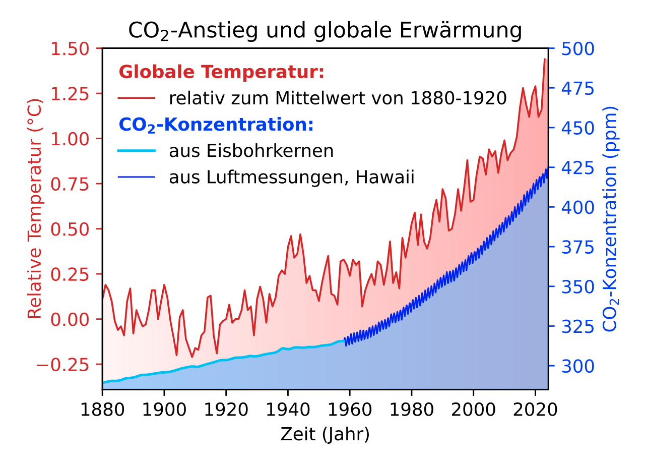
Global warming and raise of the CO2 concentration
Summary
edit
| Description |
Deutsch: Globale Erwärmung und Anstieg der CO2-Konzentration |
| Date | |
| Source | Own work |
| Author | Physikinger |
| SVG development | This plot was created with Matplotlib. |
| Source code | Python codeimport numpy, scipy.spatial
import matplotlib.pyplot as plt
from matplotlib.colors import LinearSegmentedColormap
year_T = {
# https://data.giss.nasa.gov/gistemp/tabledata_v4/GLB.Ts+dSST.txt
# GLOBAL Land-Ocean Temperature Index in 0.01 degrees Celsius base period: 1951-1980
# sources: GHCN-v4 1880-07/2021 + SST: ERSST v5 1880-07/2021
# using elimination of outliers and homogeneity adjustment
# Divide by 100 to get changes in degrees Celsius (deg-C).
# Year J-D (annual mean Temperature Jan to Dec)
1880: -16, 1881: -8, 1882: -11, 1883: -17, 1884: -28,
1885: -33, 1886: -31, 1887: -36, 1888: -17, 1889: -10,
1890: -35, 1891: -22, 1892: -27, 1893: -31, 1894: -30,
1895: -22, 1896: -11, 1897: -11, 1898: -27, 1899: -17,
1900: -8, 1901: -15, 1902: -28, 1903: -37, 1904: -47,
1905: -26, 1906: -22, 1907: -38, 1908: -43, 1909: -48,
1910: -43, 1911: -44, 1912: -36, 1913: -34, 1914: -15,
1915: -14, 1916: -36, 1917: -46, 1918: -30, 1919: -28,
1920: -27, 1921: -19, 1922: -29, 1923: -27, 1924: -27,
1925: -22, 1926: -11, 1927: -22, 1928: -20, 1929: -36,
1930: -16, 1931: -9, 1932: -16, 1933: -29, 1934: -13,
1935: -20, 1936: -15, 1937: -3, 1938: 0, 1939: -2,
1940: 13, 1941: 19, 1942: 7, 1943: 9, 1944: 20,
1945: 9, 1946: -7, 1947: -3, 1948: -11, 1949: -11,
1950: -17, 1951: -7, 1952: 1, 1953: 8, 1954: -13,
1955: -14, 1956: -19, 1957: 5, 1958: 6, 1959: 3,
1960: -3, 1961: 6, 1962: 3, 1963: 5, 1964: -20,
1965: -11, 1966: -6, 1967: -2, 1968: -8, 1969: 5,
1970: 3, 1971: -8, 1972: 1, 1973: 16, 1974: -7,
1975: -1, 1976: -10, 1977: 18, 1978: 7, 1979: 16,
1980: 26, 1981: 32, 1982: 14, 1983: 31, 1984: 16,
1985: 12, 1986: 18, 1987: 32, 1988: 39, 1989: 27,
1990: 45, 1991: 40, 1992: 22, 1993: 23, 1994: 31,
1995: 45, 1996: 33, 1997: 46, 1998: 61, 1999: 38,
2000: 39, 2001: 53, 2002: 63, 2003: 62, 2004: 53,
2005: 67, 2006: 63, 2007: 66, 2008: 54, 2009: 65,
2010: 72, 2011: 61, 2012: 65, 2013: 67, 2014: 74,
2015: 90, 2016: 101, 2017: 92, 2018: 85, 2019: 97,
2020: 102, 2021: 85, 2022: 89, 2023: 117
}
year_Temperature, Temperature = (numpy.array(list(x()), dtype='d') for x in (year_T.keys, year_T.values))
Temperature = Temperature / 100
year1 = 1880
# Keeling curve, monthly data, taken at Mauna Loa, Observatory, Hawaii
#
# C. D. Keeling, et al., Exchanges of atmospheric CO2 and 13CO2 with
# the terrestrial biosphere and oceans from 1978 to 2000.
# I. Global aspects, SIO Reference Series, No. 01-06,
# Scripps Institution of Oceanography, San Diego, 88 pages, 2001.
#
# https://scrippsco2.ucsd.edu/data/atmospheric_co2/mlo.html
# data from https://scrippsco2.ucsd.edu/assets/data/atmospheric/stations/in_situ_co2/monthly/monthly_in_situ_co2_mlo.csv
with open("monthly_in_situ_co2_mlo.csv", 'r') as f:
t, ppm_Keeling = [], []
for line in f:
if not line.startswith('"') and not line.startswith(' '):
data = line.split(',')
val = float(data[8])
if val > 0:
t.append(float(data[3]))
ppm_Keeling.append(val)
year_Keeling, ppm_Keeling = map(numpy.array, (t, ppm_Keeling))
# CO2 concentration from ice core measurements
# Rubino et al. 2013, https://agupubs.onlinelibrary.wiley.com/doi/full/10.1002/jgrd.50668
# Colum 1: effective age [AD] for CO2
# Colum 2: CO2 corrected for blank and gravity [ppm]
#
CO2_ice_core = [
[1993.0, 354.31], [1993.0, 353.58], [1991.0, 352.5], [1991.0, 352.33], [1991.0, 351.83],
[1990.0, 351.14], [1990.0, 350.72], [1990.0, 350.57], [1989.0, 349.53], [1989.0, 349.02],
[1988.0, 347.6], [1987.0, 345.44], [1987.0, 345.14], [1987.0, 344.97], [1987.0, 344.51],
[1987.0, 344.25], [1986.0, 344.28], [1986.0, 343.66], [1986.0, 343.64], [1986.0, 342.88],
[1986.0, 342.8], [1985.0, 342.53], [1985.0, 341.57], [1983.0, 339.52], [1983.0, 339.41],
[1979.0, 335.23], [1979.0, 334.47], [1976.0, 332.37], [1996.0, 359.62], [1996.0, 359.67],
[1996.0, 359.65], [1994.0, 357.35], [1994.0, 356.96], [1994.0, 357.02], [1994.0, 357.09],
[1992.0, 353.86], [1992.0, 353.66], [1992.0, 353.65], [1992.0, 353.73], [1989.0, 350.05],
[1989.0, 349.8], [1989.0, 349.78], [1989.0, 349.58], [1983.0, 341.58], [1983.0, 341.16],
[1983.0, 341.42], [1983.0, 341.15], [1971.0, 324.9], [1971.0, 324.88], [1971.0, 325.04],
[1971.0, 324.8], [1957.0, 316.44], [1957.0, 316.29], [1957.0, 316.33], [1957.0, 316.24],
[1938.0, 312.5], [1938.0, 312.58], [1938.0, 312.23], [1938.0, 312.31], [1938.0, 312.07],
[1938.0, 312.28], [1998.0, 361.78], [2001.0, 368.0], [2001.0, 368.04], [1929.0, 305.84],
[1929.0, 305.23], [1929.0, 305.39], [1929.0, 305.37], [1929.0, 305.16], [1929.0, 305.3],
[1962.0, 316.59], [1972.0, 330.35], [1977.0, 335.55], [1977.0, 332.37], [1956.0, 314.46],
[1956.0, 315.54], [1956.0, 316.04], [1969.0, 323.87], [1969.0, 324.09], [1969.0, 320.38],
[1974.0, 331.55], [1950.0, 312.0], [1967.0, 320.49], [1972.0, 328.42], [1965.0, 319.2],
[1965.0, 319.89], [1971.0, 326.31], [1971.0, 326.65], [1970.0, 324.56], [1964.0, 319.12],
[1969.0, 325.54], [1963.0, 319.07], [1969.0, 325.08], [1963.0, 319.78], [1963.0, 317.45],
[1940.0, 309.8], [1963.0, 317.45], [1962.0, 319.14], [1962.0, 317.52], [1938.0, 308.48],
[1967.0, 322.17], [1960.0, 313.09], [1966.0, 320.98], [1959.0, 316.33], [1958.0, 316.1],
[1958.0, 314.57], [1957.0, 315.27], [1929.0, 305.78], [1957.0, 314.24], [1957.0, 314.64],
[1928.0, 305.67], [1955.0, 314.83], [1955.0, 314.6], [1961.0, 318.21], [1954.0, 313.17],
[1954.0, 312.8], [1954.0, 312.75], [1954.0, 311.69], [1959.0, 311.98], [1952.0, 312.18],
[1950.0, 313.66], [1949.0, 309.69], [1948.0, 311.57], [1947.0, 313.21], [1947.0, 312.52],
[1906.0, 299.63], [1946.0, 312.56], [1945.0, 311.28], [1945.0, 310.22], [1902.0, 297.14],
[1944.0, 312.36], [1942.0, 311.62], [1942.0, 312.14], [1942.0, 312.74], [1942.0, 312.05],
[1941.0, 307.74], [1941.0, 311.8], [1947.0, 310.36], [1946.0, 311.97], [1945.0, 311.81],
[1939.0, 311.04], [1939.0, 311.39], [1939.0, 312.36], [1939.0, 308.55], [1945.0, 310.44],
[1893.0, 295.32], [1938.0, 310.66], [1938.0, 312.38], [1937.0, 307.06], [1937.0, 307.76],
[1936.0, 309.52], [1936.0, 309.17], [1942.0, 311.9], [1942.0, 313.78], [1936.0, 307.26],
[1935.0, 306.32], [1934.0, 306.76], [1934.0, 306.63], [1934.0, 307.84], [1884.0, 289.23],
[1940.0, 310.95], [1933.0, 305.94], [1933.0, 308.28], [1932.0, 308.26], [1938.0, 311.94],
[1931.0, 305.72], [1931.0, 305.76], [1929.0, 305.71], [1928.0, 307.62], [1928.0, 308.42],
[1934.0, 309.63], [1868.0, 287.99], [1925.0, 305.32], [1925.0, 304.62], [1923.0, 306.13],
[1923.0, 307.7], [1923.0, 303.14], [1923.0, 307.82], [1923.0, 303.18], [1920.0, 301.88],
[1925.0, 304.72], [1919.0, 304.61], [1918.0, 303.44], [1918.0, 303.67], [1918.0, 304.06],
[1918.0, 304.24], [1851.0, 288.79], [1916.0, 301.92], [1914.0, 301.07], [1914.0, 300.33],
[1847.0, 286.84], [1913.0, 301.3], [1911.0, 299.26], [1911.0, 297.73], [1911.0, 298.11],
[1910.0, 297.87], [1837.0, 284.15], [1909.0, 301.5], [1833.0, 283.82], [1906.0, 297.33],
[1905.0, 299.02], [1904.0, 295.99], [1827.0, 285.91], [1825.0, 281.36], [1902.0, 295.26],
[1902.0, 294.44], [1900.0, 294.22], [1899.0, 297.05], [1899.0, 295.28], [1814.0, 284.43],
[1894.0, 293.81], [1894.0, 293.17], [1893.0, 294.86], [1892.0, 295.17], [1890.0, 290.92],
[1889.0, 292.38], [1889.0, 292.3], [1799.0, 281.23], [1799.0, 284.37], [1887.0, 294.34],
[1796.0, 280.4], [1796.0, 282.3], [1886.0, 288.12], [1794.0, 281.62], [1884.0, 289.76],
[1883.0, 292.46], [1880.0, 287.77], [1780.0, 273.07], [1877.0, 289.33], [1779.0, 280.24],
[1874.0, 291.56], [1873.0, 286.66], [1773.0, 277.86], [1870.0, 286.33], [1870.0, 287.99],
[1868.0, 289.83], [1868.0, 289.24], [1764.0, 276.4], [1867.0, 284.71], [1867.0, 285.4],
[1763.0, 277.16], [1864.0, 286.65], [1863.0, 285.35], [1752.0, 276.46], [1752.0, 278.0],
[1862.0, 287.17], [1749.0, 277.6], [1859.0, 286.63], [1857.0, 283.16], [1741.0, 276.81],
[1855.0, 285.57], [1854.0, 288.05], [1734.0, 278.31], [1851.0, 285.47], [1850.0, 284.0],
[1723.0, 277.01], [1723.0, 278.27], [1846.0, 282.79], [1846.0, 284.45], [1845.0, 283.18],
[1844.0, 283.53]]
year_ice, ppm_ice = numpy.array(CO2_ice_core).T
# Calculate temperature trend
# nPoly = 4
# phi = numpy.array([year_Temperature**i for i in range(nPoly)])
# A = phi @ phi.T
# b = phi @ Temperature
# c = numpy.linalg.solve(A, b)
# yPoly = c @ phi
tRef0, tRef1 = 1880, 1920
TMargin = 0.18
CO2Min, CO2Max = 285, 500
TemperaturReference = numpy.mean(Temperature[(year_Temperature >= tRef0) & (year_Temperature < tRef1)])
TemperatureShifted = Temperature - TemperaturReference
numpy.mean(TemperatureShifted[year_Temperature<1920])
# Ice core data smoothing from scattered data
# Covariance model according to Reference:
# C. E. Rasmussen & C. K. I. Williams, Gaussian Processes for Machine Learning, the MIT Press,
# 2006, <span lang="en" dir="ltr">[[:en:ISBN|<span lang="en" dir="ltr">ISBN</span>]]</span> [[Special:BookSources/026218253X|026218253X]], 2006 Massachusetts Institute of Technology. www.GaussianProcess.org/gpml
# Section 5.4.3 Examples and Discussion
#
# Here we ignore k2, since the ice core data have
# no seasonal cycle.
def k1(d,p1=66,p2=67): return p1**2*numpy.exp(-d**2/(2*p2**2))
def k2(d,p3=2.4,p4=90,p5=1.3): return p3**2*numpy.exp(-d**2/(2*p4**2) - 2*numpy.sin(numpy.pi*d)**2/p5**2)
def k3(d,p6=0.66,p7=1.2,p8=0.78): return p6*(1+d**2/(2*p8*p7**2))**(-p8)
def k4(d,p9=0.18,p10=1.6): return p9**2*numpy.exp(-d**2/(2*p10**2))
def kNoise(p11=0.19): return p11**2
covFunc = lambda d: k1(d) + k3(d) + k4(d)
def covMat(x1, x2, covFunc, noise=0): # Covariance matrix
cov = covFunc(scipy.spatial.distance_matrix(numpy.atleast_2d(x1).T, numpy.atleast_2d(x2).T))
if not noise==0: cov += numpy.diag(numpy.zeros(len(x1)) + noise)
return cov
x_known = year_ice
y_known = ppm_ice
m = numpy.mean(y_known) # Parameter in Reference 341
nDivideYear = 4
x_unknown = numpy.arange(1880*nDivideYear, year_Keeling[0]*nDivideYear) / nDivideYear
Ckk = covMat(x_known, x_known, covFunc, noise=1)
Cuu = covMat(x_unknown, x_unknown, covFunc)
CkkInv = numpy.linalg.inv(Ckk)
Cuk = covMat(x_unknown, x_known, covFunc)
covPost = Cuu - numpy.dot(numpy.dot(Cuk,CkkInv),Cuk.T)
y_unknown = numpy.dot(numpy.dot(Cuk,CkkInv),y_known - m) + m
year_reconstructed = x_unknown
ppm_reconstructed = y_unknown
year_Total = numpy.concatenate([year_reconstructed, year_Keeling])
ppm_Total = numpy.concatenate([ppm_reconstructed, ppm_Keeling])
# Plot the figure
fig = plt.figure(figsize=(5.0,3.6))
TMin = numpy.min(TemperatureShifted) - TMargin
plt.title('CO${}_2$-Anstieg und globale Erwärmung') # %i - %i'%(year1, year_Temperature[-1])
axTemp = plt.gca()
axTemp.tick_params(axis='y', colors='C3')
axCO2 = plt.gca().twinx()
axCO2.tick_params(axis='y', colors='#0040F0')
polygon = axTemp.fill_between(year_Temperature, TMin, TemperatureShifted, color='none')
# axTemp.plot(year_Temperature, yPoly - TemperaturReference, 'r--', label='Trend')
p1, = axTemp.plot(year_Temperature, TemperatureShifted, 'C3-', linewidth=1, markersize=3, label=f'Globale Temperatur, relativ zum\nMittelwert von {tRef0} - {tRef1}')
axCO2.fill_between(year_Total, CO2Min, ppm_Total, color='#70B0FF', alpha=0.6)
p2, = axCO2.plot(year_Keeling, ppm_Keeling, '-', color='#0020F0', linewidth=0.8, label='CO${}_2$-Konzentration\n(Luftmessung, Hawaii)')
p3, = axCO2.plot(year_reconstructed, ppm_reconstructed, '-', color='#00C0F0', linewidth=1.4, label='CO${}_2$-Konzentration\n(aus Eisbohrkernen)')
cm = LinearSegmentedColormap.from_list("Custom", [(1, 0.96, 0.96), (1, 0.68, 0.68)], N=256//4)
verts = numpy.vstack([p.vertices for p in polygon.get_paths()])
gradient = axTemp.imshow(numpy.linspace(0, 1, 256//4)[None,:], cmap=cm, aspect='auto',
extent=[verts[:, 0].min(), verts[:, 0].max(), verts[:, 1].min(), verts[:, 1].max()])
gradient.set_clip_path(polygon.get_paths()[0], transform=axTemp.transData)
plt.xlabel('Jahr')
axTemp.set_ylabel('Relative globale Temperatur (°C)', color='C3')
axCO2.set_ylabel('CO${}_2$-Konzentration (ppm)', color='#0040F0')
axTemp.yaxis.set_label_coords(-0.13, 0.53)
axTemp.set_ylim(None,1.5)
axTemp.set_ylim(TMin,None)
axCO2.set_ylim(CO2Min,CO2Max-0)
plt.xlim(year1, year_Temperature[-1]+1)
axTemp.legend([p1, p3, p2], [i.get_label() for i in [p1,p3,p2]], frameon=False)
plt.tight_layout()
# plt.show()
plt.savefig('Globale_erwärmung.svg')
|
Licensing
edit
I, the copyright holder of this work, hereby publish it under the following license:
| This file is made available under the Creative Commons CC0 1.0 Universal Public Domain Dedication. | |
| The person who associated a work with this deed has dedicated the work to the public domain by waiving all of their rights to the work worldwide under copyright law, including all related and neighboring rights, to the extent allowed by law. You can copy, modify, distribute and perform the work, even for commercial purposes, all without asking permission.
|
File history
Click on a date/time to view the file as it appeared at that time.
| Date/Time | Thumbnail | Dimensions | User | Comment | |
|---|---|---|---|---|---|
| current | 08:03, 21 June 2024 | | 480 × 346 (129 KB) | Physikinger (talk | contribs) | Legend, noise assumption |
| 22:25, 20 June 2024 |  | 480 × 346 (127 KB) | Physikinger (talk | contribs) | With ice core data | |
| 22:52, 17 June 2024 |  | 480 × 346 (241 KB) | Physikinger (talk | contribs) | Uploaded own work with UploadWizard |
You cannot overwrite this file.
File usage on Commons
There are no pages that use this file.
File usage on other wikis
The following other wikis use this file:
- Usage on de.wikipedia.org