File:Planet that has 90 obliquity temperature through the year 2 1 1 1.png

Original file (972 × 631 pixels, file size: 241 KB, MIME type: image/png)
Captions
Captions
Summary
edit
| Description |
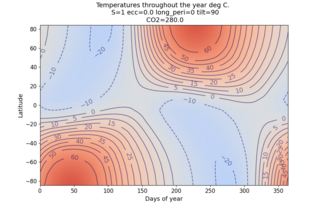
English: Planet that has 90 obliquity - temperature through the year |
| Date | |
| Source | Own work |
| Author | Merikanto |
Python3 source code
-
- temperatures, if S=0.93*S0
- sun radiation down 7% from current.
- python3/climlab code
-
- 23.10.2023 0000.0004e
import numpy as np
import matplotlib.pyplot as plt
from matplotlib import cm
import climlab
from climlab import constants as const
from climlab.process.diagnostic import DiagnosticProcess
from climlab.domain.field import Field, global_mean
def plot_temp_section(model, timeave=True):
   fig = plt.figure()
   ax = fig.add_subplot(111)
   #viridis = cm.get_cmap('jet')
   #viridis = cm.get_cmap('turbo')
   #viridis = cm.get_cmap('winter')
   viridis = cm.get_cmap('cool_r')
   #viridis = cm.get_cmap('PuBu')
   plt.set_cmap(viridis)
   if timeave:
       field = model.timeave['Tatm'].transpose()
   else:
       field = model.Tatm.transpose()
   levels1=[-90,-80,-70,-60,-50,-40,-30,-20,-10,0,10,20,30,40,50,60,70,80,90,100]
   cax = ax.contourf(model.lat, model.lev,field-273.15, levels=200)
   CS = ax.contour(model.lat, model.lev,field-273.15,levels=levels1,
                colors='k'  # negative contours will be dashed by default
                )
   ax.clabel(CS,fmt='%1.1f',fontsize=14, inline=1)
   ax.invert_yaxis()
   ax.set_title("Temperature profile", fontsize=18)
   ax.set_xlabel("Latitude", fontsize=15)
   ax.set_ylabel("Pressure", fontsize=15)
   ax.xaxis.set_tick_params(labelsize=14)
   ax.yaxis.set_tick_params(labelsize=14)
   ax.set_xlim(-90,90)
   ax.set_xticks([-90, -60, -30, 0, 30, 60, 90])
   #cbar1=fig.colorbar(cax)
   #cbar1.ax.tick_params(labelsize=15)
class tanalbedo(DiagnosticProcess):
   def __init__(self, **kwargs):
       super(tanalbedo, self).__init__(**kwargs)
       self.add_diagnostic('albedo')
       Ts = self.state['Ts']
       self._compute_fixed()
   def _compute_fixed(self):
       Ts = self.state['Ts']
       try:
           lon, lat = np.meshgrid(self.lon, self.lat)
       except:
           lat = self.lat
       phi = lat
       try:
           albedo=np.zeros(len(phi));
           albedo=0.42-0.20*np.tanh(0.052*(Ts-3))
       except:
           albedo = np.zeros_like(phi)
       dom = next(iter(self.domains.values()))
       self.albedo = Field(albedo, domain=dom)
   def _compute(self):
       self._compute_fixed()
return {}
- main code
num_years=1
rau=1.0 ## planet a au
S1_base=1361.5 ## current
- insok=1/(rau*rau) ## insolation coefficient"
insok=1 ## OK 0.93
- insok=1.0
albedo=0.3 ## constant albedo OK , but not stepper
- albedo=0.06
- co2=1*120/1e6
- co2=180/1e6
co2=280/1e6
- ecc= 0.0167643
- long_peri=280.32687
- obliquity=23.459277
ecc=0.0
long_peri=0
obliquity=90
waterdepth1=50
cloudiness=0.0
waterdepth=10
S1_abs=S1_base*insok
title1='Temperatures throughout the year deg C. \n S='+str(round(insok,3))+" ecc="+str(round(ecc,3))+" long_peri="+str(round(long_peri,1))   +" tilt="+str(round(obliquity,2))+ "\n CO2="+str(co2*1e6)
- orbit1={'ecc': 0.0167643, 'long_peri': 280.32687, 'obliquity': 23.459277, 'S0':S1_abs}
- orbit1={'ecc': 0.3, 'long_peri': 0, 'obliquity': 60, 'S0':S1_abs}
orbit1={'ecc': ecc, 'long_peri': long_peri, 'obliquity': obliquity, 'S0':S1_abs}
print(rau, insok)
- not used
delta_t = 60. * 60. * 24. * 30
absorber_vmr = {'CO2':co2,
               'CH4':800./1e9,
               'N2O':100./1e9,
               'O2':0.21,
               'CFC11':1./1e9,
               'CFC12':1./1e9,
               'CFC22':1./1e9,
               'CCL4':1./1e9,
               'O3':1./1e6}
- state = climlab.column_state(num_lev=20, num_lat=1, water_depth=5.)
state = climlab.column_state(num_lev=8, num_lat=16, water_depth=waterdepth)
insol = climlab.radiation.DailyInsolation(name='Insolation',
domains=state['Ts'].domain, S0=S1_abs, orb=orbit1)
- insol.S0=S1_abs
h2o = climlab.radiation.ManabeWaterVapor(state=state, relative_humidity=1.0)
rad = climlab.radiation.CAM3(name='Radiation', state=state,
return_spectral_olr=True,
icld=cloudiness,
S0 = S1_abs,
insolation=insol.insolation,
coszen=insol.coszen,
absorber_vmr = absorber_vmr,
albedo=albedo
)
print(insol.S0)
print (insol.coszen)
- quit(-1)
conv = climlab.convection.ConvectiveAdjustment(name='Convective Adjustment',state=state, adj_lapse_rate=6.5)
rcm = climlab.couple([insol, rad,conv,h2o], name='RCM')
surface = rcm.domains['Ts']
rcm.water_depth=waterdepth1
rcm.Tf=10
- quit(-1)
- rad.a0=albedo
- WARNING DYNAMIC ALBEDO NOK
rcm.remove_subprocess('albedo')
- alb = climlab.surface.albedo.StepFunctionAlbedo(state=rcm.state, Tf=-10, **rcm.param)
- alb = climlab.surface.albedo.ConstantAlbedo(domains=surface, **rcm.param)
- alb.albedo[:]=albedo
- alb = tanalbedo(state=rcm.state, **rcm.param)
- rcm.add_subprocess('albedo', alb)
- print (alb.diagnostics)
- quit(-1)
print(" Integrate ...")
rcm.integrate_years(1)
- Create and exact clone of the previous model
diffmodel = climlab.process_like(rcm)
diffmodel.name = 'Seasonal RCE with heat transport'
- thermal diffusivity in W/m**2/degC
- D = 0.05
D=0.0001
- meridional diffusivity in m**2/s
K = D / diffmodel.Tatm.domain.heat_capacity[0] * const.a**2
print("K ", K)
d = climlab.dynamics.MeridionalDiffusion(K=K, state={'Tatm': diffmodel.Tatm}, **diffmodel.param)
diffmodel.add_subprocess('Meridional Diffusion', d)
- diffmodel = climlab.couple([rad,conv,h2o, insol,d], name='Seasonal diffmodel')
print(diffmodel)
- diffmodel.integrate_years(1)
diffmodel.integrate_years(num_years)
- diffmodel.integrate_converge()
tatm2=state['Tatm']-273.15
print(tatm2)
print("Plot ")
- plot_temp_section(rcm, timeave=True)
- plot_temp_section(diffmodel, timeave=True)
- plot_temp_section(diffmodel, timeave=True)
tlayer1=tatm2[...,7].ravel()
tlayer2=tatm2[...,7].ravel()
- print (" Tatmlen",len(tlayer1))
tlayer1=np.nan_to_num(tlayer1)
tlayer2=np.nan_to_num(tlayer2)
meantemp=np.mean(tlayer1)
meantemp2=np.mean(tlayer2)
print(tlayer1)
print(tlayer2)
print(" meantemp A ",meantemp)
print(" meantemp B ",meantemp2)
- fig, ax = plt.subplots(dpi=100)
- state['Tatm'].to_xarray().plot(ax=ax, y='lev', yincrease=False)
- state['Tatm'].to_xarray().plot(ax=ax,x='lat', y='lev', yincrease=False)
tatm=state['Tatm']-273.15
rcm=diffmodel
years=1
num_steps_per_year = int(rcm.time['num_steps_per_year'])
Tyear = np.empty((rcm.lat.size, num_steps_per_year*years))
for m in range(num_steps_per_year*years):
    rcm.step_forward()
    Tyear[:,m] = np.squeeze(rcm.Ts)
Tmin=np.min(Tyear)
Tmax=np.max(Tyear)
tmean1=np.mean(Tyear[:,:])
print("Tmean ", tmean1-273.15)
print("Tmin ", Tmin-273.15)
print("Tmax ", Tmax-273.15)
fig = plt.figure(figsize=(5,5))
ax = fig.add_subplot(111)
factor = 365. / num_steps_per_year
- cmap1=plt.cm.seismic
- cmap1=plt.cm.winter
- cmap1=plt.cm.cool_r
- cmap1=plt.cm.cool
- cmap1=plt.cm.seismic
- cmap1=plt.cm.RdYlBu_r
- cmap1=plt.cm.turbo_r
- cmap1=plt.cm.jet
cmap1=plt.cm.coolwarm
- cmap1=cmap1.reversed()
- levels1=[-80,-70,-60,-50,-40,-30]
levels2=[-250,-200,-150,-100,-80,-70,-65,-60,-55,-50,-45,-40,-35,-30,-20,-10,0,5,10,15,20,25,30,35,40,45,50,60,80,90,100,120,150,200,250,300,500,1000,2000,4000]
cax = ax.contourf(factor * np.arange(num_steps_per_year*(years-1), num_steps_per_year*years),
   rcm.lat, Tyear[:,:]-273.15,
   cmap=cmap1, vmin=-100, vmax=100, levels=255)
cs1 = ax.contour(factor * np.arange(num_steps_per_year*(years-1),num_steps_per_year*years),
   rcm.lat, Tyear[:,:]-273.15,
   colors='#00005f', alpha=0.5, vmin=Tmin, vmax=Tmax, levels=levels2)
ax.clabel(cs1, cs1.levels, inline=True, fontsize=14)
- cbar1 = plt.colorbar(cax)
ax.set_title(title1, fontsize=14)
ax.tick_params(axis='x', labelsize=12)
ax.tick_params(axis='y', labelsize=12)
ax.set_xlabel('Days of year', fontsize=13)
ax.set_ylabel('Latitude', fontsize=13)
plt.show()
- plt.savefig('1000dpi.png', dpi=1000)
- print(rcm)
- quit(-1)
- plot_temp_section(rcm, timeave=True)
- plt.imshow(tatm)
- ax.set_xlabel("Temperature (K)")
- ax.set_ylabel("Pressure (hPa)")
- ax.grid()
- plt.plot()
- plt.show()
Licensing
edit
| This file is made available under the Creative Commons CC0 1.0 Universal Public Domain Dedication. | |
| The person who associated a work with this deed has dedicated the work to the public domain by waiving all of their rights to the work worldwide under copyright law, including all related and neighboring rights, to the extent allowed by law. You can copy, modify, distribute and perform the work, even for commercial purposes, all without asking permission.
|
File history
Click on a date/time to view the file as it appeared at that time.
| Date/Time | Thumbnail | Dimensions | User | Comment | |
|---|---|---|---|---|---|
| current | 18:56, 12 November 2023 | | 972 × 631 (241 KB) | Merikanto (talk | contribs) | Uploaded own work with UploadWizard |
You cannot overwrite this file.
File usage on Commons
There are no pages that use this file.