Soul windsurfer
| This user has uploaded images to Wikimedia Commons. |
|}
| Babel user information | |||||||||
|---|---|---|---|---|---|---|---|---|---|
| |||||||||
| Users by language | |||||||||
| Babel user information | |||||||||
|---|---|---|---|---|---|---|---|---|---|
| |||||||||
| Users by language | |||||||||
| Babel user information | |||||||||
|---|---|---|---|---|---|---|---|---|---|
| |||||||||
| Users by language | |||||||||
![]() Wikipedia - my page in wiki
Wikipedia - my page in wiki
home page. - dead but web archive can help
https://tools.wmflabs.org/glamtools/glamorous.php
Wikibooks -en - Adam majewski
Mathematics Stack Exchange MathOverflow Wikibooks -pl - Adam majewski

|
The Photographer's Barnstar |
| foto |
| This file was selected as the media of the day for 06 March 2012. It was captioned as follows:
English: Quadratic Julia set with Internal level sets for c values along internal ray 0 of main cardioid of Mandelbrot set
Other languages
English: Quadratic Julia set with Internal level sets for c values along internal ray 0 of main cardioid of Mandelbrot set Македонски: Квадратно Жулиино множество со множества на внатрешно ниво за вредностите на c, заедно со внатрешен зрак 0 на главната кардоида од Манделбротово множество. 中文(简体):朱利亚集合
|
syntaxhighlight edit
{{Galeria
|Nazwa = Trzy krzywe w różnych skalach
|wielkość = 400
|pozycja = right
|Plik:LinLinScale.svg|Skala liniowo-liniowa
|Plik:LinLogScale.svg|Skala liniowo-logarytmiczna
|Plik:LogLinScale.svg|Skala logarytmiczno-liniowa
|Plik:LogLogScale.svg|Skala logarytmiczno-logarytmiczna
}}


== c source code==
<syntaxhighlight lang="c">
</syntaxhighlight>

== bash source code==
<syntaxhighlight lang="bash">
</syntaxhighlight>


==make==
<syntaxhighlight lang=makefile>
all:
	chmod +x d.sh
	./d.sh
</syntaxhighlight>


Tu run the program simply

  make


==text output==
<pre>

==references==
<references/>

| Other versions = {{vva}}
| Other fields = {{Created with code|+=Source code|h1=none|e1=Created using {{W|Maxima (software)|Maxima}}.|l1=gnuplot|c1=   }}

|other fields={{Igen|Matplotlib|+|code=  }}
function edit
| Description | Function displaying a cusp at (0,1) |
|---|---|
| Equation | |
| Co-ordinate System | Cartesian |
| X Range | -4 .. 4 |
| Y Range | -0 .. 3 |
| Derivative | |
| Points of Interest in this Range | |
| Minima | |
| Cusps | |
| Derivatives at Cusp | ,
|


The program can calculate many of the objects found in Singularity theory:
- Algebraic curves defined by a single polynomial equation in two variables. e.g. a circle x^2 + y^2 - r^2;
- Algebraic surfaces defined by a single polynomial equation in three variables. e.g. a cone x^2 + y^2 - z^2;
- Paramertised curves defined by a 3D vector expression in a single variable. e.g. a helix [cos(pi t), sin(pi t), t];
- Parameterised surfaces defined by a 3D vector expression in two variables. e.g. a cross-cap [x,x y,y^2];
- Intersection of surfaces with sets defined by an equation. Can be used to calculate non-polynomial curves.
- Mapping from R^3 to R^3 defined by 3D vector equation in three variables. e.g. a rotation [cos(pi th) x - sin(pi th) y,sin(pi th) x + cos(pi th) y,z];
- Intersections where the equation depends on the definition of another curve or surface. e.g. The profile of a surface N . [A,B,C]; N = diff(S,x) ^^ diff(S,y);
- Mappings where the equation depends on another surface. For example projection of a curve onto a surface.
- Intersections where the equations depends on a pair of curves. For example the pre-symmetry set of a curve.
- Mapping where the equation depends on a pair of curves. For example the Symmetry set.
video edit
formats edit
YT:
- .MOV
- .MPEG-1 ( also commons)
- .MPEG-2 ( also commons)
- .MPEG4
- .MP4
- .MPG
- .AVI ( also commons)
- .WMV
- .MPEGPS
- .FLV
- 3GPP
- WebM ( also commons)
- DNxHR
- ProRes
- CineForm
- HEVC (h265)
commmons:
tools edit
Kodeki
Text
Image guidelines edit
- Commons:Image_guidelines
- :Category:Images_by_technical_criteria
- :Category:Color in computer graphics
- :Commons:Featured pictures
FIles
LCD tests edit
commons edit
{{ValiCat|+|type=stop}}

[[Category:CommonsRoot]]
Help:
- Commons:Categories#Category_names
- Category:CommonsRoot
- Category:Categories
- https://meta.wikimedia.org/wiki/Namespace
- Commons:Categories#How_to_categorize:_guidance_by_topic
- Commons:Categories#Sorting_categories
- essays
Category edit
Image
- Static
- non-photographic
- computer graphic
- art
- AI
- human
Criteria for fractals classifications
- by method
- by fractal type
- by country ???
- by year ( ? creation ?)
- by File type ( or file format)
- static image
- raster
- vector
- animation
- video
- static image
- by quality
- by technical citeria
- by features
- Fractal images - media of the day
Help
spike edit
- "spike function" x -> 1 - exp(a*abs(mod(x,1)-0.5)^b)
- periodic version of function f can be created by reducing mod 1: fp(x)=f(x−⌊x⌋)
- Exponential_decay
- https://zone.ni.com/reference/en-XX/help/371361R-01/gmath/spike_function/#details
It can be used for:
- highlight the boundary ( 1D)
- Specular reflection in Phong reflection model ( 3D )
peak edit
- https://fractalforums.org/programming/11/cellular-coloring-of-mandelbrot-insides/3264
- https://stackoverflow.com/questions/3684484/peak-detection-in-a-2d-array
- enriched signal regions = peak
-
- Matlabs peak function: The peaks function is useful for demonstrating graphics functions, such as contour, mesh, pcolor, and surf.
- It is obtained by translating and scaling Gaussian distributions.
- Matlab's peaks function has three peaks, three valleys and three saddle points.

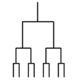
tree edit
slope edit
// "Psychofract" by Carlos Ureña - 2015
// License Creative Commons Attribution-NonCommercial-ShareAlike 3.0 Unported License.


mat3 tran1,
     tran2 ; //transform matrix for each branch

const float pi = 3.1415926535 ;

const float rsy = 0.30 ; // length of each tree root trunk in NDC

// -----------------------------------------------------------------------------

mat3 RotateMat( float rads )
{
   float c = cos(rads),
         s = sin( rads ) ;

   return mat3(  c,  s, 0.0,
                -s,   c, 0.0,
               0.0, 0.0, 1.0  );
}
// -----------------------------------------------------------------------------

mat3 TranslateMat( vec2 d )
{
   return mat3(  1.0, 0.0, 0.0,
                 0.0, 1.0, 0.0,
                 d.x, d.y, 1.0 );
}
// -----------------------------------------------------------------------------

mat3 ScaleMat( vec2 s )
{
   return mat3( s.x, 0.0, 0.0,
                0.0, s.y, 0.0,
                0.0, 0.0, 1.0 );
}
// -----------------------------------------------------------------------------

mat3 ChangeFrameToMat( vec2 org, float angg, float scale )
{
   float angr = (angg*pi)/180.0 ;
   return
        ScaleMat( vec2( 1.0/scale, 1.0/scale ) )
      * RotateMat( -angr )
      * TranslateMat( -org ) ;
}
// -----------------------------------------------------------------------------

float RectangleDistSq( vec3 p )
{
   if ( 0.0 <= p.y && p.y <= rsy )
       return p.x * p.x;

   if (p.y > rsy)
       return p.x*p.x + (p.y-rsy)*(p.y-rsy) ;

   return p.x*p.x + p.y*p.y ;
}
// -----------------------------------------------------------------------------

float BlendDistSq( float d1, float d2, float d3 )
{
   float dmin = min( d1, min(d2,d3)) ;

   return 0.5*dmin ;
}
// -----------------------------------------------------------------------------

vec4 ColorF( float distSq, float angDeg )
{
   float b = min(1.0, 0.1/(sqrt(distSq)+0.1)),
         v = 0.5*(1.0+cos( 200.0*angDeg/360.0 + b*15.0*pi ));

   return vec4( b*b*b,b*b,0.0,distSq) ; // returns squared distance in alpha component
}
// -----------------------------------------------------------------------------

float Trunk4DistSq( vec3 p )
{
   float d1 = RectangleDistSq( p );

   return d1 ;
}

// -----------------------------------------------------------------------------

float Trunk3DistSq( vec3 p )
{
   float d1 = RectangleDistSq( p ),
         d2 = Trunk4DistSq( tran1*p ),
         d3 = Trunk4DistSq( tran2*p );

   return BlendDistSq( d1, d2, d3 ) ;
}

// -----------------------------------------------------------------------------

float Trunk2DistSq( vec3 p )
{
   float d1 = RectangleDistSq( p ),
         d2 = Trunk3DistSq( tran1*p ),
         d3 = Trunk3DistSq( tran2*p );

   return BlendDistSq( d1, d2, d3 ) ;
}

// -----------------------------------------------------------------------------

float Trunk1DistSq( vec3 p )
{
   float d1 = RectangleDistSq( p ) ,
         d2 = Trunk2DistSq( tran1*p ),
         d3 = Trunk2DistSq( tran2*p );

   return BlendDistSq( d1, d2, d3 ) ;
}

// -----------------------------------------------------------------------------

float Trunk0DistSq( vec3 p )
{
   float d1 = RectangleDistSq( p ) ,
         d2 = Trunk1DistSq( tran1*p ),
         d3 = Trunk1DistSq( tran2*p );

   return BlendDistSq( d1, d2, d3 ) ;
}
// -----------------------------------------------------------------------------
// compute the color and distance to tree, for a point in NDC coords

vec4 ComputeColorNDC( vec3 p, float angDeg )
{
   vec2 org = vec2(0.5,0.5) ;
   vec4 col = vec4( 0.0, 0.0, 0.0, 1.0 );
   float dmin ;

   for( int i = 0 ; i < 4 ; i++ )
   {
      mat3 m = ChangeFrameToMat( org, angDeg + float(i)*90.0, 0.7 );
   	  vec3 p_transf = m*p ;
      float dminc = Trunk0DistSq( p_transf ) ;

      if ( i == 0 )
         dmin = dminc ;
      else if ( dminc < dmin )
         dmin = dminc ;
   }
   return ColorF( dmin, angDeg ); // returns squared dist in alpha component
}
// -----------------------------------------------------------------------------

vec3 ComputeNormal( vec3 p, float dd, float ang, vec4 c00 )
{
   vec4   //c00  = ComputeColorNDC( p, ang )  ,
         c10  = ComputeColorNDC( p + vec3(dd,0.0,0.0), ang )  ,
         c01  = ComputeColorNDC( p + vec3(0.0,dd,0.0) , ang ) ;
   float h00  = sqrt(c00.a),
         h10  = sqrt(c10.a),
         h01  = sqrt(c01.a);
   vec3  tanx = vec3( dd, 0.0, h10-h00 ),
         tany = vec3( 0.0, dd, h01-h00 );
   vec3  n    = normalize( cross( tanx,tany ) );

   if ( n.z < 0.0 ) n *= -1.0 ;
   return n ;
}

// -----------------------------------------------------------------------------

void mainImage( out vec4 fragColor, in vec2 fragCoord )
{

   const float width = 0.1 ;


   vec2  res  = iResolution.xy ;
   float mind = min(res.x,res.y);
   vec2  pos  = fragCoord.xy ;
   float x0   = (res.x - mind)/2.0 ,
         y0   = (res.y - mind)/2.0 ,
         px   = pos.x - x0 ,
         py   = pos.y - y0 ;


   // compute 'tran1' and 'tran2':

   vec2  org1      = vec2( 0.0, rsy ) ;
   float ang1_deg  = +20.0 + 30.00*cos( 2.0*pi*iTime/4.05 ),
         scale1    = +0.85 +  0.40*cos( 2.0*pi*iTime/2.10 )  ;

   vec2  org2      = vec2( 0.0, rsy ) ;
   float ang2_deg  = -30.0 + 40.00*sin( 2.0*pi*iTime/2.52 ),
         scale2    = +0.75 +  0.32*sin( 2.0*pi*iTime/4.10 )  ;

   tran1 = ChangeFrameToMat( org1, ang1_deg, scale1 ) ;
   tran2 = ChangeFrameToMat( org2, ang2_deg, scale2 ) ;

   // compute pixel color (pixCol)

   float mainAng = 360.0*iTime/15.0 ,    // main angle, proportional to time
         dd      = 1.0/float(mind) ;           // pixel width or height in ndc
   vec3  pixCen  = vec3( px*dd, py*dd, 1.0 ) ; // pixel center
   vec4  pixCol  = ComputeColorNDC( pixCen, mainAng ),
         resCol  ;

   // compute output color as a function 'use_normal'

    const bool use_gradient = true ;

   if ( use_gradient )
   {
      vec3 nor     = ComputeNormal( pixCen, dd, mainAng, pixCol );
      vec4 gradCol = vec4( max(nor.x,0.0), max(nor.y,0.0), max(nor.z,0.0), 1.0 ) ;

      resCol = 0.8*pixCol+ 0.2*gradCol ;
   }
   else
      resCol = pixCol ;


   fragColor = vec4( resCol.rgb, 1.0 ) ;
}
curves edit
rays edit
- Quadratic Julia set with Internal binary decomposition for internal ray 0.ogv
- mob-tree-256.png from Arithmetic Exponential Generating Functions by Linas Vepstas
- analytic functions of interest in number theory in C by Linas
- Tree roots by Naoki Tsutae in openprocessing
- A LEVEL 3, WEIGHT 32 TRACEFORM by David Lowry-Duda
- ModularForm
- btree by dahart
- BinaryTreeVar
- desmos - binary decomposition
- Fractal surprise from complex function iteration Posted on February 28, 2013 by Peter Stampfli - Processing code
// https://geometricolor.wordpress.com/2013/02/28/fractal-surprise-from-complex-function-iteration-the-code/
//Fractal surprise from complex function iteration: The code Posted on February 28, 2013 by Peter Stampfli
//  here is the program for the last post:  Fractal surprise from complex function iteration
//   simply use it in processing 1.5 (I don’t know if it works in the new version 2.)
// you can download it from processing.org


float range, c,step;
int n, iter, count;
float rsqmax;

void setup() {
size(600, 600);
c=0.4;
step=0.002;
iter=40;
rsqmax=100;
range=1.2;
count=0;
}

void draw() {
int i, j, k;
float d=2*range/width;
float x, y, h;
float phi, phiKor;                             //  phiKor is the trivial phase change to subtract
colorMode(HSB, 400, 100, 100);
loadPixels();
for (j=0;j<height;j++) {
for (i=0;i
y=-range+d*j;
x=-range+d*i;
phiKor=0;
for (k=0;k<iter;k++) {
if (x*x+y*y>rsqmax) {
break;
}
phiKor+=atan2(y, x);
h=x*x-y*y+c;
y=2*x*y;
x=h;
}
phi=atan2(y, x)-phiKor;    //  correction
phi=0.5*phi/PI;
phi=(phi-floor(phi))*2*PI;  //  calculate phase phi mod 2PI
pixels[i+j*width]=color(phi/PI*200, 100, 100);
}
}
updatePixels();
//  saveFrame(“a-####.jpg”);
println(count+” “+c);
c-=step;
if (c<0) {
noLoop();
}
count++;
}

pins=[]
pins_num=150

setup=()=> {
  createCanvas(windowWidth, windowHeight)
  y=0
  for (i=0; i<pins_num; i++ ) {
    pins[i]=createVector(random(width), random(height))
  }
}

draw=()=> {
  if (y<height) {
    for (x=0; x<width; x++ ) {
      angle=0
      pins.forEach(p=>angle+=atan2(p.y-y, p.x-x))
      colour=map(sin(angle), -1, 1, 0, 256)
      stroke(colour)
      line(x, y, x, y+colour)
    }
    y++
  }
}

mousePressed=()=>setup()

in the circle edit
- https://www.shadertoy.com/view/Xdt3z7
- https://www.ma.imperial.ac.uk/~dcheragh/Teaching/2016-F-GCA/2016-F-GCA.pdf
- pufferfish create elaborate circular nests


_%3D_z%5E2.png)

strip edit
void mainImage( out vec4 col, in vec2 k)
{
    k.x += iResolution.x * 8. * (1. - cos(iTime * 0.05));
    col = vec4(int(k / 2.) & 1 << int(k.y / 30.) );

}
- binary tiling
-

-
-
-

-


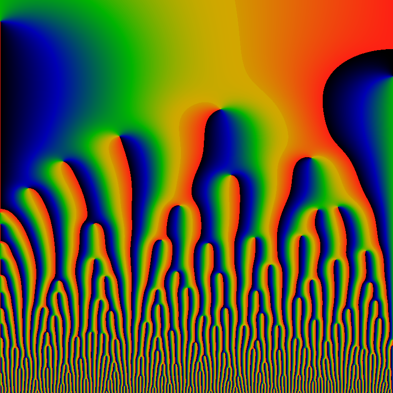
The field lines edit
In a Fatou domain (that is not neutral) there is a system of lines orthogonal to the system of equipotential lines, and a line of this system is called a field line.
If we colour the Fatou domain according to the iteration number (and not the real iteration number), the bands of iteration show the course of the equipotential lines, and so also the course of the field lines.
If the iteration is towards ∞, we can easily show the course of the field lines, namely by altering the colour according to whether the last point in the sequence is above or below the x-axis, but in this case (more precisely: when the Fatou domain is super-attracting) we cannot draw the field lines coherently (because we use the argument of the product of for the points of the cycle).

For an attracting cycle C, the field lines issue from the points of the cycle and from the (infinite number of) points that iterate into a point of the cycle. And the field lines end on the Julia set in points that are non-chaotic (that is, generating a finite cycle).
Let
- r be the order of the cycle C
- z* be a point in C.
- (the r-fold composition)
- the complex number by


If the points of C are , is the product of the r numbers . The real number 1/ is the attraction of the cycle, and our assumption that the cycle is neither neutral nor super-attracting, means that 1 < 1/ < ∞. The point z* is a fixed point for , and near this point the map has (in connection with field lines) character of a rotation with the argument of (so that ).


colour the Fatou domain edit
In order to colour the Fatou domain, we have chosen a small number and set the sequences of iteration to stop when , and we colour the point z according to


- the number k which gives Level Set Method (LSM)
- the real iteration number, if we prefer a smooth colouring
FL edit
def
- the field lines, which are the lines orthogonal to the equipotential lines
- A field line is orthogonal to the equipotential surfaces, which are the loci for the points of constant iteration number
The colouring is determined by
- the distance to the centre line of the field line (density/across)
- and by the potential function (density/along),
This colouring can be mixed with the colouring of the background. As two colour scales are required, these must be imported.
The field lines are determined by their number,
- their (relative) thickness (≤ 1)
- a number transition determining the mixing of the colours of the field lines with the background - e.g
- . 0.1 for a soft transition and therefore indistinct and thinner looking field lines,
- 4 for more well defined field lines.
If the field lines do not run precisely coherently, the bailout number must be diminished and the maximum iteration number increased. Here is the function 1 1 0 0 1, and the background is made of one colour by setting the density to 0:
Within a field line there are two local distances:
- the distance from the centre line
- the distance from the equipotential line.
In addition there are two whole numbers:
- the number of the field line
- the iteration number.
The two local distances establish local coordinate systems within the field lines, and this means that it is possible to colour on the basis of mathematical procedures or pictures that are input.
And the two whole numbers mean that such procedures or pictures can be made to depend on the field line number and the iteration number.
When the Fatou domain is associated to a super-attracting cycle, the field lines cannot be drawn coherently.
However, it is possible to draw a system of bands that follow their courses, but the number of which increases for each increase in the iteration number. If the function is a polynomial (that is, if the denominator is a constant), the factor of increase is the degree of the polynomial. For a general rational function the factor is the difference between the degree of the numerator and the denominator, but the constellation of the partitions is not regular, because fiels lines also originate from the points that are zeros of the denominator, and from the (infinitely many) points that are iterated into one of these zeros.
For the function z4/(1 + z), the field lines are separated in three, but field lines also come from the point -1 and the points iterated into -1:
colouring of the field lines edit
If we choose a direction from z* given by an angle , the field line issuing from z* in this direction consists of the points z such that the argument of the number satisfies the condition


- .

For if we pass an iteration band in the direction of the field lines (and away from the cycle), the iteration number k is increased by 1 and the number is increased by , therefore the number is constant along the field line.

A colouring of the field lines of the Fatou domain means that we colour the spaces between pairs of field lines: we use the name field line for such coloured "interval of field lines", As a field line in our terminology is an interval of field lines
we choose a number of regularly situated directions issuing from z*, and in each of these directions we choose two directions around this direction. As it can happen, that the two bounding field lines do not end in the same point of the Julia set, our coloured field lines can ramify (endlessly) in their way towards the Julia set. We can colour on the basis of the distance to the centre line of the field line, and we can mix this colouring with the usual colouring.
Let n be the number of field lines and let t be their relative thickness (a number in the interval [0, 1]). For the point z, we have calculated the number , and z belongs to a field line if the number (in the interval [0, 1]) satisfies |v - i/n| < t/(2n) for one of the integers i = 0, 1, ..., n, and we can use the number |v - i/n|/(t/(2n)) (in the interval [0, 1] - the relative distance to the centre of the field line) to the colouring.

Where
- an attracting cycle C
- r be the order of the cycle C
- the points of C are
- z* be a point in C;
- it is a fixed point of
- the argument of the number


Pictures edit
- In the first picture, the function is of the form and we have only coloured a single Fatou domain
- The second picture shows that field lines can be made very decorative (the function is of the form ).
- third picture: A (coloured) field line is divided up by the iteration bands, and such a part can be put into a ono-to-one correspondence with the unit square: the one coordinate is the relative distance to one of the bounding field lines, this number is (v - i/n)/(t/(2n)) + 1/2, the other is the relative distance to the inner iteration band, this number is the non-integral part of the real iteration number. Therefore we can put pictures into the field lines. As many as we desire, if we index them according to the iteration number and the number of the field line. However, it seems to be difficult to find fractal motives suitable for placing of pictures - if the intention is a picture of some artistic value. But we can restrict the drawing to the field lines (and possibly introduce transparency in the inlaid pictures), and let the domain outside the field lines be another fractal motif


-
 Field lines. the function is of the form and we have only coloured a single Fatou domain
 -
 Field lines. the function is of the form
 -
 Pictures inlaid in Field lines


smoke edit
relief edit
Cartographic
Hachures, are a form of shading using lines
Sketchy
with lines
define the colors used for different terrain heights:
map projections edit
Digital Image Processing edit
- data analysis
- image processing
- image enhacement = process an image so that result is more suitable than original image for specific application
- Histogram equalization
- image enhacement = process an image so that result is more suitable than original image for specific application
computer graphic edit
- https://matlabsimulation.com/image-preprocessing-projects/
- http://learn.graphics/
- https://www.cs.cmu.edu/~kmcrane/
- https://perso.liris.cnrs.fr/david.coeurjolly/teaching/ENS2018/c-gd-contour.html
- https://www.tankonyvtar.hu/en/tartalom/tamop425/0046_algorithms_of_informatics_volume2/ch10.html
- http://math.hws.edu/graphicsbook/index.html
- www.pling.org.uk/cs/cgv.html
- www.tutorialspoint.com/computer_graphics/computer_graphics_curves.htm
- github.com/jagregory/abrash-black-book
- pages.mtu.edu/~shene/COURSES/cs3621/NOTES/model/b-rep.html
- pages.mtu.edu/~shene/COURSES/cs3621/NOTES/notes.html
libraries edit
icc edit
- http://www.imagemagick.org/Usage/formats/#profiles
- https://stackoverflow.com/questions/18272797/converting-rgb-to-cmyk-using-icc-profile
convert image_rgb.tiff -profile "RGB.icc" -profile "CMYK.icc" image_cmyk.tiff
algorithm edit
perceptually accurate rendering algorithm:
- Render your image using correct radiometric calculations. You trace individual wavelengths of light or buckets of wavelengths. Whatever. In the end, you have an image that has a representation of the spectrum received at every point.
- At each pixel, you take the spectrum you rendered, and convert it to the CIE XYZ color space. This works out to be integrating the product of the spectrum with the standard observer functions (see CIE XYZ definition).
- This produces three scalar values, which are the CIE XYZ colors.
- Use a matrix transform to convert this to linear RGB, and then from there use a linear/power transform to convert linear RGB to sRGB.
- Convert from floating point to uint8 and save, clamping values out of range (your monitor can't represent them).
- Send the uint8 pixels to the framebuffer.
- The display takes the sRGB colors, does the inverse transform to produce three primaries of particular intensities. Each scales the output of whatever picture element it is responsible for. The picture elements light up, producing a spectrum. This spectrum will be (hopefully) a metamer for the original spectrum you rendered.
- You perceive the spectrum as you would have perceived the rendered spectrum.
hdr edit
- Set your ISO to 200, set your camera to Aperture Priority
- take three photos with exposure settings as EV 0, EV-2, and EV+2. The more differently exposed photos you have, the better.
- Merge to HDR
- Select 32-bit/channel and tick Remove Ghosts
- . Click Image > Mode > 16-bit/channel
- tone mapping. Adjust the settings depending on how you want your HDR photo to look.
image enhancement techniques edit
- gray-level transformation functions
- linear (negative and identity transformations)
- logarithmic (log and inverse-log transformations)
- power-law (nth power and nth root transformations).T
bit depth and bitrate edit
- 8-bit = 2^8 = 256 values. 256 to create an 8-bit grayscale image
- 16-bit grayscale. This means that they capture over 65,000 shades of gray. [1]
- 24 bit = with three colour channels, that’s 256 (red) x 256 (green) x 256 (blue) for a total of around 2^8^3 = 16.7 million individual colours (RGB = true color) 16 777 216 = 256^3 = 2^8^3
aliasing edit
- "A simple way to prevent aliasing of cosine functions (the color palette in this case) by removing frequencies as oscillations become smaller than a pixel. You can think of it as an LOD system. Move the mouse to compare naive versus band-limited cos(x)" Inigo Quilez
Gimp edit
- flatpak run org.gimp.GIMP
Commons edit
- Category:Images_by_technical_criteria
- Commons:Maximum file size
- Commons:File captions
- Commons:Structured data
- Commons:Image_guidelines
- Commons:Quality_images
- https://journals.aas.org/graphics-guide/
- Commons:Graphics village pump
- https://commonshelper.toolforge.org/
- svg optimizers
Template edit
nested squares edit
float SCALE, RAD;
int VECT = 1;

void setup() {
  size(640, 640);
  rectMode(CENTER);
  noStroke();
}

void draw() {
  background(0);
  translate(width/2, height/2);
  int i = frameCount*2 % width;
  if (i==0) VECT = -VECT;
  SCALE = dist(i, 0, 0, width-i)/width;
  RAD = atan2(width-i, i*VECT);
  for (int j=0; j<16; j++) {
    scale(SCALE);
    rotate(RAD);
    fill(map(j, 0, 15, 64, 255));
    rect(0, 0, width, height);
  }
}
conformal edit
- http://www.madore.org/~david/weblog/d.2013-11-11.2166.application-conforme.html
- https://gist.github.com/adammaj1/d7ce0351b7e3c98336f4a9fdcd9b33a3#file-ellipse-conformal-map-sage
# Square of eccentricity (but not that of the drawn ellipse):
modparm = 3/4

# The size of the drawn ellipse (semimajor and semiminor) is computed
# below.

### Mapping the inside of the disk to the inside of the ellipse:

prescale = N(modparm^(-1/4))
postscale = N(pi/(2*elliptic_kc(modparm)))

# The conformal map taking the unit disk in CC to the inside of the
# ellipse, and 0 to 0:
def phi(z):
    z = N(z)
    t = N(asin(CC(z*prescale)))
    u = N(elliptic_f(t, modparm))
    return N(sin(postscale*u))

# A memoized version of phi, for efficiency:
phi_tab = {}
def memoize_phi(z):
    z = N(z)
    if z in phi_tab:
        return phi_tab[z]
    phi_tab[z] = phi(z)
    return phi_tab[z]

# Convenience function for plotting phi(rad*exp(2*I*pi*ang)):
def plothelp(rad, ang):
    return memoize_phi(rad*exp(2*I*pi*ang))

def plothelp_x(rad, ang):
    return real(plothelp(rad,ang))

def plothelp_y(rad, ang):
    return imag(plothelp(rad,ang))

circplots = [parametric_plot([lambda t: plothelp_x(i/10, t), lambda t: plothelp_y(i/10, t)], (0,1)) for i in range(11)]
radplots = [parametric_plot([lambda t: plothelp_x(t, i/24), lambda t: plothelp_y(t, i/24)], (0,1)) for i in range(24)]
# sum(circplots + radplots)

### Mapping the outside of the disk to the outside of the ellipse:

#semimajor = real(phi(1))
#semiminor = imag(phi(I))
semimajor = N(cosh((pi/4)*elliptic_kc(1-modparm)/elliptic_kc(modparm)))
semiminor = N(sinh((pi/4)*elliptic_kc(1-modparm)/elliptic_kc(modparm)))

# The conformal map taking the complement of the unit disk in CC to
# the complement of the ellipse, and infinity to infinity:
def phi2(z):
    z = N(z)
    return N(((semimajor+semiminor)/2)*z + ((semimajor-semiminor)/2)/z)

# Convenience function for plotting phi2(rad*exp(2*I*pi*ang)):
def plothelp2(rad, ang):
    return phi2(rad*exp(2*I*pi*ang))

def plothelp2_x(rad, ang):
    return real(plothelp2(rad,ang))

def plothelp2_y(rad, ang):
    return imag(plothelp2(rad,ang))

circplots2 = [parametric_plot([lambda t: plothelp2_x(1+i/10, t), lambda t: plothelp2_y(1+i/10, t)], (0,1), color="red") for i in range(11)]
radplots2 = [parametric_plot([lambda t: plothelp2_x(t, i/24), lambda t: plothelp2_y(t, i/24)], (1,2), color="red") for i in range(24)]
sum(circplots + radplots + circplots2 + radplots2)
log-polar mapping edit
- Complex Logarithmic Mapping. Concentric circles in the z-plane are mapped into vertical lines in the w-plane and radial lines in the z-plane are mapped into horizontal lines in the w-plane (Fig. 1). The image produced in the w-plane is generally referred to as a logpolar mapping or logmap
examples
- An Introduction to the Log-Polar Mapping by Jorge Dias, Helder Araujo, 1996, Proceedings of 2nd Workshop on Cybernetic Vision , also from semanticscholar
- Log-spherical Mapping in SDF Raymarching by Pierre Cusa
- https://arxiv.org/pdf/1509.06344.pdf
- Finding straight lines and circles in log-polar images by David Young, University of Sussex
- https://stackoverflow.com/questions/13211595/how-can-i-convert-coordinates-on-a-circle-to-coordinates-on-a-square
- http://squircular.blogspot.com/2015/09/mapping-circle-to-square.html
- https://rghmatlabstuff.wordpress.com/2012/02/21/mapping-s-plane-to-z-plane/
- https://dspcan.homestead.com/files/Ztran/zlap.htm
- https://sthoduka.github.io/imreg_fmt/docs/log-polar-transform/
- https://stackoverflow.com/questions/7781416/find-an-inverse-log-transformation-of-an-image-in-matlab?utm_medium=organic&utm_source=google_rich_qa&utm_campaign=google_rich_qa
- https://www.foerstemann.name/dokuwiki/doku.php?id=log_z_-mandelbrot-zooms
- http://users.isr.ist.utl.pt/~alex/Projects/TemplateTracking/logpolar.htm
- Rapid Anisotropic Diffusion Using Space-Variant Vision: complex log transformation for various values of the map parameter a. Note that decreasing a (moving from left to right) increases the representation of the foveal region in the log plane. Dark areas correspond to regions outside the domain of the mapping.
- https://www.researchgate.net/publication/257641946_A_novel_quantum_representation_for_log-polar_images_Quantum_Inf
- https://www.youtube.com/watch?v=v_0otkcYY18
- STRIATE CORTEX: ADVANCED PIXEL MANIPULATION by Amnon on August 21, 2011
mapping edit
- Twisted Mandelbrot Set „Let p is pixel location relative to image's center. Normally, c = c0 + p. Twisted, c = c0 + p^2.” and you change c0 along some circle to get the rotation ?
Exponential map [2]
- exponential_mapping_with_kalles_fraktaler by Claude Heiland-Allen
- Exponential map From the Mandelbrot Set Glossary and Encyclopedia, by Robert Munafo
- feigenbaum stretch by Claude Heiland-Allen
- wolfram Exp function visualizations
- Interactive Decal Compositing with Discrete Exponential Maps
- Polar and Log-Polar Transformations in scikit-image python
- escher droste math by B. de Smit and H. W. Lenstra Jr.
- FRACTALS IN POLAR COORDINATES by Mika Seppä
- mapping of represents the map of the complex plane. It maps the positive half plane to the complex plane minus the negative real axis.


notation edit

is meant to say is a map whose domain is A and whose codomain is B. A and B are both sets. E.g.


means $\text{sq}$ is a real valued function defined over the real numbers.
If you have , then we also have the notation where

- a is an element of A
- and b is an element of B.
This can be used to fix the notation for the evaluation of the map: E.g. .

You can also prescript the actual map in that moment, by defining what , e.g.


Other use for this notation is to simply say to what element of B a particular is mapped to. E.g. .


To do edit
- http://functions.wolfram.com/ElementaryFunctions/Exp/visualizations/4/ShowAll.html
- http://functions.wolfram.com/ElementaryFunctions/Log/visualizations/4/
- https://www.chebfun.org/examples/complex/ConformalVis.html
- http://paulbourke.net/fractals/septagon/?fbclid=IwAR0finOMTmkd18jN8eq0rC5x8PKfIY7Lxy6yIjPlLnbw-oXcyRhg1a-MavE
spiral edit
- on the parameter plane
- on the dynamic plne
- component of Julia set near fixed point fractalforums.org: shaping-spirals
- arm consisted from many components ( renormalizabel ? ) like https://commons.wikimedia.org/wiki/File:Julia_set_for_f(z)_%3D_z%5E2%2B0.355534_-0.337292*i.png
- external rays landing on the fixed point
- critical orbit
- component of Julia set near fixed point fractalforums.org: shaping-spirals
Mandelbrot edit
- Technical Descriptions: Mandelbrot Fractals of z0 = 0.1 on p-Canvases Top Left: Centered at p = (3.567150, 0.002194); Top Right: p = (3.567174, 0.002195) Bottom: p = (3.570063528376, 0.00000001192) Generated by the Logistic Equation https://www.sekinoworld.com/fractal/
- The Misiurewicz point with preperiod k = 23 and period n = 2 is near c = -0.7756837680090538+0.13646736829469008i https://www.youtube.com/watch?v=6DTBaNOZXlU center of spiral
- rays are wiggly, here is one of period 20, with external angle .(00000000001111111111)
- Real: -0.4804138344396693204232547058 Imaginary: 0.5326479652407472622369935790 Size: 0.000000000003637978 (4.0 includes the diameter of the first Mandelbrot iteration.) The size can be converted to zoom by using the formula: zoom = 4 / size. https://fractalforums.org/fractal-image-of-the-month-contest/70/iotmc-september-2023-theme-is-energy-and-the-style-is-free/5170/msg38165#new
- -1.770119403587, 0.0041109401046462
planes edit
- Formula: z = z^2 + c + a*(2^c - c^2) with z0=0 and a changing from 1.1 to 5.5 --- Morph details: Location: (3 + 0i) Magnification changes from 1.4 to 3.2 Iteration count: 250 Bailout value: 128 https://www.youtube.com/watch?v=QifOH6tf8v4 by Some dude
- https://github.com/adammaj1/Mandelbrot-Sets-Alternate-Parameter-Planes
jux edit
- center -0.029890989869028344 + 0.158824979369024322
- zoom = 10^n, n = 15.093
- max iter = 8192
- bailout = 10^3
- https://fractalforums.org/fractal-image-of-the-month-contest/70/iotmc-november-2023-themebetween-autumn-and-winter-style-free/5196/new#new
- formula sin(3z6 + 5z-6)+c, Mandelbrot mode
dense edit
- Example: c0 = -0.39055 + 0.58680 i @ 1e5 magnification, 64k iterations
- the set of all Misiurewicz points is dense on the boundary of the Mandelbrot set ( Local connectivity of the Mandelbrot set at certain infinitely renormalizable points by Yunping Jiang ) https://arxiv.org/abs/math/9508212
period edit
- 0. Assume a well-behaved formula like quadratic Mandelbrot set.
- 1. A hyperbolic component of period P is surrounded by an atom domain of period P.
- 2. The size of the atom domain is around 4x larger than a disk-like component, often larger for cardioid-like components.
- 3. Conjecture: Newton's method in 1 complex variable (f_c^P(z)-z=0) can find the limit cycle Z_1 .. Z_P when starting from the Pth iterate of 0, when c is sufficiently within the atom domain
- 4. The limit cycle has multiplier (product 2 Z_k) 0 at the center and 1 in magnitude at the boundary of the component.
- 5. The atom domain coordinate is 0 at the center and 1 in magnitude at the boundary of the atom domain.
- 6. Perturbed Newton's method can be used for deep zooms.
- 7. The limit cycle can also be used for interior distance estimation.
Start from period 1 increasing, you get a sequence of atom domains. At each, if the atom domain coordinate is small, use Newton's method to find the limit cycle. If the limit cycle has small multiplier, stop, period is detected. If the iterate escapes, stop, pixel is exterior.
22-legged ant in the m-set edit
- centered on -0.72398340 + 0.28671980i, with magnifications ranging from 0.714 to 120,000
- Rolo Silver's newsletter "Amygdala" issue 7 page 1
- I was watching this video by Rudy Rucker https://www.youtube.com/watch?v=ICrNOTQBS8U where he found an interesting structure in the m-set that he called "the 22 legged ant".
- https://fractalforums.org/noobs-corner/76/i-need-help-finding-the-22-legged-ant-in-the-m-set/4065/msg35757#msg35757
$ m-describe double 1000 1000 -0.72398340 0.28671980 1
the input point was -0.723983400000000055 + +0.286719800000000025 i
the point didn't escape after 1000 iterations

nearby hyperbolic components to the input point:

- a period 1 cardioid
  with nucleus at +0.000000000000000000 + +0.000000000000000000 i
  the component has size 1 and is pointing west
  the atom domain has size 0
  the nucleus domain coordinate is 0 at turn 0.000000000000000000
  the atom    domain coordinate is -nan at turn -nan
  the nucleus is 0.77869 to the east-south-east of the input point
  the input point is exterior to this component at
  radius 1.0354 and angle 0.45522 (in turns)
  a point in the attractor is -0.497319450905372551 + +0.143745216108897733 i
  external angles of this component are:
  .(0)
  .(1)

- a period 2 circle
  with nucleus at -1.000000000000000000 + +0.000000000000000000 i
  the component has size 0.5 and is pointing west
  the atom domain has size 1
  the nucleus domain coordinate is 1.2361 at turn 0.500000000000000000
  the atom    domain coordinate is 1 at turn 0.000000000000000000
  the nucleus is 0.39799 to the south-west of the input point
  the input point is exterior to this component at
  radius 1.5919 and angle 0.12803 (in turns)
  a point in the attractor is -0.861857110872783827 + +0.396178203198002954 i
  external angles of this component are:
  .(01)
  .(10)

- a period 105 cardioid
  with nucleus at -0.723948838355664148 + +0.286852337885451558 i
  the component has size 3.7103e-07 and is pointing east-south-east
  the atom domain has size 0.00010235
  the nucleus domain coordinate is 1.5924 at turn 0.128053542315208269
  the atom    domain coordinate is 0.39811 at turn 0.128053542315208269
  the nucleus is 0.00013697 to the north-north-east of the input point
  external angles of this component are:
  .(010101010011010010101010100101010101001010101010010101010100101010101001010101010010101010100101010101001)
  .(010101010011010100101010101001010101010010101010100101010101001010101010010101010100101010101001010101010)

- a period 116 cardioid
  with nucleus at -0.723983481008419805 + +0.286719746468555081 i
  the component has size 1.7465e-07 and is pointing east-south-east
  the atom domain has size 7.0286e-05
  the nucleus domain coordinate is 36.617 at turn 0.370795651751681277
  the atom    domain coordinate is 0.73603 at turn 0.878154585895997375
  the nucleus is 9.7098e-08 to the west-south-west of the input point
  the input point is interior to this component at
  radius 0.83522 and angle 0.62253 (in turns)
  a point in the attractor is +0.000065706660165846 + -0.000227325037589120 i
  the interior distance estimate is 4.491e-08
  external angles of this component are:
  .(01010101001101001010101010010101010100101010101001010101010010101010100101010101001010101010010101010100101010101001)
  .(01010101001101010010101010100101010101001010101010010101010100101010101001010101010010101010100101010101001010101010)

nearby Misiurewicz points to the input point:

- 2p1
  the strength is 0.38133
  the center is at -2.000000000000000000 + 0.000000000000000000 i
  the center is 1.3078 to the west-south-west of the input point
  the multiplier has radius 4 and angle 0.00000 (in turns)

- 3p1
  the strength is 0.35938
  the center is at -1.543689012692076368 + -0.000000000000000000 i
  the center is 0.8684 to the west-south-west of the input point
  the multiplier has radius 1.6786 and angle -0.50000 (in turns)

- 12p1
  the strength is 0.00037767
  the center is at -0.724112682973573563 + 0.286456567676711404 i
  the center is 0.00029327 to the south-south-west of the input point
  the multiplier has radius 1.0354 and angle 0.45526 (in turns)

- 12p11
  the strength is 2.0286e-05
  the center is at -0.724112682973573563 + 0.286456567676711460 i
  the center is 0.00029327 to the south-south-west of the input point
  the multiplier has radius 1.4656 and angle 0.00789 (in turns)

- 2p116
  the strength is 2.3938e-14
  the center is at -0.723874171053648929 + 0.286847598521453362 i
  the center is 0.00016812 to the north-east of the input point
  the multiplier has radius 41405 and angle -0.45166 (in turns)

- 3p116
  the strength is 9.1963e-15
  the center is at -0.723892769678345482 + 0.286784362650608693 i
  the center is 0.00011128 to the north-east of the input point
  the multiplier has radius 8827.5 and angle 0.13635 (in turns)

$ cabal repl # while in folder with mandelbrot prelude project
...
ghci> fmap Txt.plain . Sym.angledAddress . Sym.rational =<< Txt.parse ".(01010101001101001010101010010101010100101010101001010101010010101010100101010101001010101010010101010100101010101001)"
Just "1_5/11->11_1/2->22_1/2->33_1/2->44_1/2->55_1/2->66_1/2->77_1/2->88_1/2->99_1/2->110_1/2->116"


alg by Claude edit
coloured with atom domain quadrant, exterior binary decomposition, and interior and exterior distance estimates) Double precision, no perturbation. Atom domain coordinate is smallest z divided by previous smallest z. Check for interior only if the atom domain coordinate is small (I think the smallest atom domains are for circle-like components, and are about 4x the size of the component, cardioid-like components tend to have much larger atom domains). Atom domain quadrant colouring is based on the quadrant of the atom domain coordinate, something like floor(4 * arg(a)/2pi).
Here's my inner loop and supporting functions: https://code.mathr.co.uk/mandelbrot-graphics/blob/49377e6bc8a034403b26b79ee1c53f7a6c328a21:/c/lib/m_d_compute.c#l75 https://code.mathr.co.uk/mandelbrot-numerics/blob/6a23adebed4f3793d2b64ef32ce1b7ccfec3230c:/c/lib/m_d_interior_de.c#l8 https://code.mathr.co.uk/mandelbrot-numerics/blob/6a23adebed4f3793d2b64ef32ce1b7ccfec3230c:/c/lib/m_d_attractor.c#l8
How many iterations do you perform for distance estimation?
For exterior distance estimation, you need a large escape radius, eg 100100.
For interior distance estimation, you need the period, then a number (maybe 10 or so should usually be enough) Newton steps to find the limit cycle.
Iteration count limit is arbitrary, with a finite limit some pixels will always be classified as "unknown".
Looks like your code is finding interior unexpectedly (points that should be exterior are falsely determined to be interior). But without seeing the source it's hard to tell.
extern bool m_d_compute_step(m_d_compute *px, int steps) {
76 if (! px) {
77 return false;
78 }
79 if (px->tag != m_unknown) {
80 return true;
81 }
82 double er2 = px->er2;
83 double _Complex c = px->c;
84 double _Complex z = px->z;
85 double _Complex dc = px->dc;
86 double _Complex zp = px->zp;
87 double _Complex zq = px->zq;
88 double mz2 = px->mz2;
89 double mzq2 = px->mzq2;
90 int p = px->p;
91 int q = px->q;
92 for (int i = 1; i <= steps; ++i) {
93 dc = 2 * z * dc + 1;
94 z = z * z + c;
95 double z2 = cabs2(z);
96 if (z2 < mzq2 && px->filter && px->filter->accept && px->filter->accept(px->filter, px->n + i))
97 {
98 mzq2 = z2;
99 q = px->n + i;
100 zq = z;
101 }
102 if (z2 < mz2) {
103 double atom_domain_radius_squared = z2 / mz2;
104 mz2 = z2;
105 p = px->n + i;
106 zp = z;
107 if (atom_domain_radius_squared <= 0.25) {
108 if (px->bias == m_interior) {
109 double _Complex dz = 0;
110 double de = -1;
111 if (m_d_interior_de(&de, &dz, z, c, p, 64)) {
112 px->tag = m_interior;
113 px->p = p;
114 px->z = z;
115 px->dz = dz;
116 px->zp = zp;
117 px->de = de;
118 return true;
119 }
120 } else {
121 if (px->partials && px->np < px->npartials) {
122 px->partials[px->np].z = z;
123 px->partials[px->np].p = p;
124 px->np = px->np + 1;
125 }
126 }
127 }
128 }
129 if (! (z2 < er2)) {
130 px->tag = m_exterior;
131 px->n = px->n + i;
132 px->p = p;
133 px->q = q;
134 px->z = z;
135 px->zp = zp;
136 px->zq = zq;
137 px->dc = dc;
138 px->de = 2 * cabs(z) * log(cabs(z)) / cabs(dc);
139 return true;
140 }
141 }
142 if (px->bias != m_interior && px->partials) {
143 for (int i = 0; i < px->np; ++i) {
144 z = px->partials[i].z;
145 zp = z;
146 int p = px->partials[i].p;
147 double _Complex dz = 0;
148 double de = -1;
149 if (m_d_interior_de(&de, &dz, z, c, p, 64)) {
150 px->tag = m_interior;
151 px->p = p;
152 px->z = z;
153 px->dz = dz;
154 px->zp = zp;
155 px->de = de;
156 return true;
157 }
158 }
159 }
160 px->tag = m_unknown;
161 px->n = px->n + steps;
162 px->p = p;
163 px->q = q;
164 px->mz2 = mz2;
165 px->mzq2 = mzq2;
166 px->z = z;
167 px->dc = dc;
168 px->zp = zp;
169 px->zq = zq;
170 return false;
171 }
mandelbrot-numerics] / c / lib / m_d_interior_de.c
1 // mandelbrot-numerics -- numerical algorithms related to the Mandelbrot set
2 // Copyright (C) 2015-2018 Claude Heiland-Allen
3 // License GPL3+ http://www.gnu.org/licenses/gpl.html
4
5 #include <mandelbrot-numerics.h>
6 #include "m_d_util.h"
7
8 extern bool m_d_interior_de(double *de_out, double _Complex *dz_out, double _Complex z, double _Complex c, int p, int steps) {
9 double _Complex z00 = 0;
10 if (m_failed != m_d_attractor(&z00, z, c, p, steps)) {
11 double _Complex z0 = z00;
12 double _Complex dz0 = 1;
13 for (int j = 0; j < p; ++j) {
14 dz0 = 2 * z0 * dz0;
15 z0 = z0 * z0 + c;
16 }
17 if (cabs2(dz0) <= 1) {
18 double _Complex z1 = z00;
19 double _Complex dz1 = 1;
20 double _Complex dzdz1 = 0;
21 double _Complex dc1 = 0;
22 double _Complex dcdz1 = 0;
23 for (int j = 0; j < p; ++j) {
24 dcdz1 = 2 * (z1 * dcdz1 + dz1 * dc1);
25 dc1 = 2 * z1 * dc1 + 1;
26 dzdz1 = 2 * (dz1 * dz1 + z1 * dzdz1);
27 dz1 = 2 * z1 * dz1;
28 z1 = z1 * z1 + c;
29 }
30 *de_out = (1 - cabs2(dz1)) / cabs(dcdz1 + dzdz1 * dc1 / (1 - dz1));
31 *dz_out = dz1;
32 return true;
33 }
34 }
35 return false;
36 }
inversion edit
- z^2 + c to z^2 + 1/c
Mandelbrot set inversion, 4 different methods in one image by Arneauxtje
First, there's the transformation from the cardioid of the body of the set to a circle. This is done in c-space (a+ib) as follows:
rho=sqrt(a*a+b*b)-1/4
phi=arctan(b/a)
a-new=rho*(2*cos(phi)-cos(2*phi))/3
b-new=rho*(2*sin(phi)-sin(2*phi))/3
Then, there's the 4 different ways on how to get from c to 1/c, that group in 3 families:
- addition: c -> c-c*t+t/c and t=0..1
- multiplication: c -> c/(t*(c*c-1)+1) and t=0..1
- exponentiation: c -> c^t and t=1..-1
The first 2 are pretty elementary to work out. The 3rd makes use of the fact that: c = a+ib = r*exp(i*phi) where r=sqrt(a*a+b*b) and phi=arctan(b/a) then c^t = r^t*exp(t*i*phi) = r^t*[cos(t*phi)+i*sin(t*phi)]
The top left is method 1, top right method 2, and the bottom 2 are variants of method 3. Hope this helps somewhat.
z_(n+1) = (z_n)^2 + (tan(t) + i*c)/(i + c*tan(t)) with t from 0.2pi to 0.35pi Another way to invert the Mandelbrot set | Closer look at t from 0.2*pi to 0.35*pi by Fraktoler Curious
structure edit
other images edit
Julia edit
Computing the Julia set of f(z) = z^2 + i where (J(f) = K(f)). [3]
- approximating the filled Julia set from above: the first 15 preimages of a large disk D = B(0, R) ⊃ K(f)
- approximating the Julia set from below: ∪0≤k≤12f−k(β) where β is a repellingfixed point in J(f) = IIM
- a good-quality picture of J(f).
- 1/(2^25) = 0.00000002980232239
- c = (6,091,023 - 19,560,658*I) * 2^-25= 0.18152663113090497 -0.58295303587653262*I
- c = 0.181502832839439 -0.582826014844503 i period = 33 center
- 0.00000002980232239×(-32,087,296 -8,265,216 *I)= -0.95627594001535744 -0.24632263185498624*I
- c = -0.808488889220256 -0.160696902421635 i period = 10000 parabolic ( 1->2 -> 8/9), periodic point z=-0.155168789522421 +0.233109501069944 *I;
- c = -0.956587955583267 -0.246201938253052 i period = 10000 ( parabolic 7/9 from 2
- 3 methods
-
 preimages of (beta)
 -
 preimages of circle


other Julia edit
- θ = 1/(10 + 1/(10 + · · ·)) Consider a polynomial P : C → C of degree d ≥ 2, with an irrationnally indifferent fixed point at the origin: P(0) = 0, P′ (0) = e 2iπθ, θ ∈ R \ Q. ( from On the linearization of degree three polynomials and Douady’s conjecture by Arnaud Ch´eritat (joint work with Xavier Buff)
- (*Koch center 3 cycle Julia*)\[IndentingNewLine]f[z_]=(-0.187-0.421*I)z^3+(-2.332-0.239*I)z^2+(-0.285+2.879*I)z+1; Roger Lee BagulaSelf-Similarity and Fractals An example of a "Koch" Julia: I was looking for an image for my new music album and found this unique Julia and re-did the picture with different colors and higher resolution: https://www.wolframcloud.com/.../j_koch9p1example2000...
- z^n + c*z where n=6, c=0.95 and R=0.2 https://geometricolor.wordpress.com/2013/10/28/coloring-the-julia-set/
- parabolic z- 32*z^5
- z3 + z + .6 I https://www.marksmath.org/scholarship/Julia.pdf
- Filled Julia set K(F) for 0 = [ai, a2, a3,...], where an = e^n. ????
- https://www.math.univ-toulouse.fr/~cheritat/GalII/galery.html
- On the Julia set of a typical quadratic polynomial with a Siegel disk By C. L. PETERSEN and S. ZAKERI
- 1/(cos(z) - z2/2) we can find this Julia set: http://www.juliasets.dk/UFP.htm GB
parabolic edit
- f(z) = z + z^4 + z^5 ( 3 petals)
sekino edit
- https://www.sekinoworld.com/fractal/
- The Julia Set of p = (0.935638029, 0.355810484) On a z-Canvas Centered at z0 = (0.5, 0) Generated by the Logistic Equation Cf. "Esmeralda Lion" in Gallery 2D
- The Julia Set of p = (0.0352236, 0.5448064) On a z-Canvas Centered at z0 = (0, 0) Generated by the Dynamical System zn+1 = zn3 + zn + p ;
- Subset of the Julia Set of p = (0.9975, 0.0752) On a z-Canvas Centered at z0 = (0.5, 0) Generated by the Logistic Equation
- Figure 0.8. "Cloisonné Elephant". Subset of the Julia Set of p = (0.971218547, 0.27795678) On a z-Canvas Centered at z0 = (0.5, 0) Generated by the Logistic Equation Cf. "Cloisonné Lion II" in Gallery 2D
- Figure 1.0(A). A Local Image of the Mandelbrot Set. Figure 2.3 is a cropped and resized image from a computer plot on the large square p-canvas with 6,400 × 6,400 pixels centered at the complex number (0.28206125, 0.011014375) with radius 0.0000011. M = 100,000 is used as the maximum number of iterations for the divergence scheme. The image contains several (deformed) replicas of the "snowman" painted black, which we call mini-Mandelbrot sets. They look like small isolated islands but as we'll find out in the next section, they are actually connected to ℳ by razor-thin "filaments" belonging to the boundary of ℳ.
- Figure 1.0(B). "Dancing Seahorses" The Julia Set of p = (-0.77146, -0.10119) On a z-Canvas Centered at z0 = (0, 0) Generated by the Mandelbrot Equation See Fractal Coloring for the Coloring Algorithm
- Figure 1.0(C). "Turquoise Lion" The Julia Set of p = (0.281215625, 0.0113825) On a z-Canvas Centered at z0 = (0, 0) Generated by the Mandelbrot Equation
- Figure 1.0(D). "Mosaic Lion" The Julia Set of p = (0.25000316315, -0.00000000895) On a z-Canvas Centered at z0 = (0, 0) Generated by the Mandelbrot Equation
- Figure 1.1(A). "Lavender Dragon" The Julia Set of p = (0.0830158, 0.5347594) On a z-Canvas Centered at z0 = (0, 0) Generated by the Dynamical System zn+1 = zn3 + zn + p
- Figure 7.9. "Pearly Elephants" Julia Fractal of q = (3.0014564, 0.08) by the Logistic Equation (7.2) The parameter p = (3.0237615, 0.1) that generates "Dancing Seahorses" shown below belongs to the orange atom of period 2 in the logistic set at Elephant Bay, hence the filled-in Julia set is painted by the convergence scheme with period index 2. Elephant bay is sandwiched by a red atom of period 1 and an orange atom of period 2, and interestingly, a parameter from the orange shore generates "seahorses" instead of "elephants."
610 edit
https://fractalforums.org/fractal-mathematics-and-new-theories/28/julia-and-parameter-space-images-of-polynomials/2786/msg16210#msg16210 marcm200 A very basic cubic Julia set p(z)=z^3+(0.099609375-0.794921875i), but with very interesting entry points into the attracting periodic cycle of length 610.
The image shows the Julia set (yellow), its attracting cycle (cyan), and some white pixels which have not (yet) entered the cycle at the current maxit of 15000 (there were much more at maxit 10000, so they will enter the cycle as expected).
I was interested to see at what point(s) the attracted numbers "enter" the cycle. Entering was defined as: If a complex number is bounded, I checked its last iterate whether it is in the attracting cycle. If so, I went backwards in the orbit until I encountered the first non-cycle point (epsilon of 10^-7). Its image was set to be the entry point.
The result was quite unambiguous. The 4k image had ~222,000 interior points, of which:
the top 3 entry points were: 0.09960906311,-0.794921357 => used 220,130 times 0.09976627035,-0.7951977228 => 251 0.09942639427,-0.7946757595 => 208
So there is a preferred point to enter the cycle - it almost looks like the not-often used entry points might be numerical errors and everything enters the cycle at the same number (or the cycle itself is a numerical error - darn, I hope my question is still valid).
Would this distribution still be accurate in the limit when one could actually test all interior points of the set and not just a finite number of rational coordinate complex numbers?
Since a point never actually goes exactly into the cycle unless it is a preimage or an image of a cycle point, but will come arbitrarily close to (some?) periodic points: Does this imply that periodic points have an event horizon - once in, never out again?
Or can an orbit point be close to a periodic point, jump out into the vicinity of another and coming closer there - and so on, so actually never getting stuck near one specific periodic point?
z^d + c edit
Internal angle = 0 ( one main component)
- d = 2 c = 1/4 = 0.25
- d = 3 c = 0.384900179459751 +0.000000000000000 i period = 10000
- d = 4 c = -0.236235196855289 +0.409171363489396 i period = 10000 ??? it should be c = 0.472464424146544;
- d = 5 c = 0.534992243981138 +0.000000000000000 i period = 10000
- d = 6 c = -0.471135846013573 +0.342300228596646 i period = 10000 ?? it should be c = 0.582559084495983 +0.000000000000000 i period = 0
Internal angle 1/3 from main component
- d = 2 c = -0.125000000000000 +0.649519052838329 i period = 10000 ( Douady rabbit )
- d = 3 c = 0.481125224324688 +0.500000000000000 i period = 10000
- d = 4 c = -0.619317130969330 +0.370556691297005 i period = 10000
- d = 5 c = 0.694975311172961 +0.267496121990569 i period = 10000
- d = 6 c = -0.719547645525888 +0.256065008698348 i period = 10000
- d = 7 c = 0.758540222557608 +0.180894796695791 i period = 10000
- d = 8 c = -0.768629397583800 +0.197192545338461 i period = 10000
cubic edit
- A 4k cubic Julia by Chris Thomasson . Here is the formula: z = pow(z, 3) - (pow(-z, 2.00001) - 1.0008875); link
- cubic
- "Let c = (.387848...) + i(.6853...). The left picture shows the filled Julia set Kc of the cubic map z3 + c, covered by level 0 of the puzzle. The center of symmetry is at 0, the point where the rays converge is α and the other fixed points are marked by dotted arrows. In this example the rotation number around α is ρα = 25 and the ray angles are 5 121 7→ 15 121 7→ 45 121 7→ 14 121 7→ 42 121 7→ 5 121 . The right picture illustrates level 1 of the puzzle for the same map. "A New Partition Identity Coming from Complex Dynamics
- Owen Maresh owen maresh(-0.4999999999999998 + 0.8660254037844387*I) - (0.2926009682749477 + 0.252068970984772*I)* z - (0.4916379276414715 + 0.2509264824918978*I)* z^2 + (0.2511839558093919 - 1.0778044459985288*I)* z^3
- f f(z)=z5+(0.8+0.8i)z4+z which has the following fixed points
- p1^=0 with multiplier |λ1|=|f′(0)|=1 (parabolic),
- p2^=−0.8−0.8i with multiplier |λ2|=|f′(−0.8−0.8i)|≈|−13.7|>1 (repelling),
- p3^=∞ with multiplier |λ3|=|limz→∞f(z)|−1=0 (super-attracting)
- f(z)=(−0.090706+0.27145i)+(2.41154−0.133695 i)z^2 − z^3 has one critical orbit attracted to an orbit of period two and one critical orbit attracted to an orbit of period three. Basic complex dynamicsA computational approach by Mark McClure
- z^3+ (0.105,0.7905); https://www.shadertoy.com/view/3llyzl
rational edit
Julia sets of rational maps ( not polynomials )
- Non-Euclidean Dreamer: It's the Julia Set of z=(1.4+1.2i)(1/(4z)-1/(z+2)), with the Break Off condition increasing throughout the Video.
- f(z) = z^3/(z^3 + 1) + c, c = 0.18 + 0.68 i
- http://www.3d-meier.de/index.html
- http://www.juliasets.dk/Ratio.htm
- 1/(z + z3)
- https://arxiv.org/pdf/1304.3881.pdf
- 1/(z^2-1)
- 1/(z^3) + the primitive 8-th root of unity : https://arxiv.org/pdf/2004.02797.pdf
- parabolic (z^3-z)/(1+4z -z^2)
- julia sets for z⁴+c/z and z²+c/z³ photoniclabs
- McMullen Maps
- The Julia sets, defined by the equation (\ref{julia}), can take all kinds of shapes, and a small change in $c$ can change the Julia set very greatly https://complex-analysis.com/content/julia_set.html
- lapin f[z]=(z^2/(c*z^2+1)) c=0.30922922123657415`-0.03212392698439477 ( pc(12)

Christopher Williams edit
- usefuljslibrary by Christopher Williams: fractals - rational_maps (*MandelbrotwithSQRT(x^2+y^2)limitedmeasure*)(*byR.L.BAGULA22.Nov2007©
Family:

Examples:
- Julia set of The most obvious feature is that it's full of holes! The fractal is homemorphic to (topologically the same as) the Sierpinski carpet
- Julia set of z2 - 1 - 0.005z-2
- f = z^2 - 0.01z^-2
- f = z2 - 0.01z-2

Phoenix formula
- z5 - 0.06iz-2
Robert L. Devaney edit
- Singular perturbations of complex polynomials

Julia sets for fc(z) = z*z + c edit
- https://www.researchgate.net/publication/315381462_The_Mandelbrot_Set_as_a_Quasi-Black_Hole
- (0.11421610355396709, 0.59570907391827810);
- (0.33751130482196073, 0.41014244936187033);
- (0.25161670227079957, 0.49833246356572231).
- (0.07023590960694610, 0.61486872535543668)
- (0.25520149659878483, 0.49473324077959746)
- (0.13811184749188554, 0.58354392530509225)
- (0.26464143869779005, 0.48473638288631671)
- (0.24725611046013074, 0.50292165702256331)
- http://www.scideveloper.com/Fractals/period.html
- mating : One polynomial is at the end of the 1/6 external ray of the Mandelbrot set, and is z->z^2+i (where i^2=-1). The other one is at the end of the 5/14 external ray and is z->z^2+c with c = -1.23922555538957 + 0.412602181602004*i
- Slow divergence in a Julia set The appearance of more diverged area (ie the purple ‘river’) in the zoom above suggests that this particular Julia set (a=−0.29609091+0.62491i)
- c = 0.280000000000000 +0.011300000000000 i period = 1 but critical orbit is interesting
- z^3 -0.040000000000000036-0.78*I, period 2 : z0= z = 0.128494244956895 -0.427153520116896 i, z1= = -0.108213690768581 -0.723219415137925 i
- z^2-0.2+0.75i, period 3
- https://de.wikipedia.org/wiki/Benutzer:Georg-Johann/Mathematik#Visualising_Julis_sets
- http://www.3d-meier.de/tut20/Julia2/Seite1.html
- expanding orbits of periodic points : http://virtualmathmuseum.org/Fractal/julia/index.html
- 0.3305 + 0.06i[4]
- 0.253930 + 0.000480i.
- 0.27310 + 0.006990i.
- Julia set c=0.763069-0.094691i
- −0.200062 + 0.807120i.
- http://yozh.org/2011/03/14/mset006/
- 0.3-0.49i
- -0.75 -0.1i ; ( outside Mandelbrot set )
- -0.7589-0.0753i http://social-biz.org/2010/03/28/generating-chaos/
- c = 0.2349 + i*0.545 fractaldesire
- c = -0.750950561621545 +0.021484356174671 i parabolic)
- http://www.multiwingspan.co.uk/vb10.php?page=frac8
- c = -0.12375 + 0.56508i
- c = -0.12 + .74 i
- c = -0.11 + 0.6557i
- c = -0.194 + 0.6557i
- c = -0.125 + 0i
-
 c=-0,75-0,14i
 -
 c=-0,75-0,14i
 -
 c=? ; IIM


const double Cx=-0.74543; const double Cy=0.11301;
-0.808 +0.174i;
-0.1 +0.651i; ( beween 1 and 3 period component of Mandelbrot set )
-0.294 +0.634i
equations for the interior of hyperbolic components edit
tuned rabbit edit
- c = 0
- 5/13
- c = -0.407104083085098 +0.584852842868102 i period = 13
- 1/2
- c = -0.410177342420846 +0.590406710726110 i period = 10000
the 5/13 Rabbit tuned with the Basilica approximates the golden Siegel disk ( LOCAL CONNECTIVITY OF THE MANDELBROT SET AT SOME SATELLITE PARAMETERS OF BOUNDED TYPE by DZMITRY DUDKO AND MIKHAIL LYUBICH )
spirals edit
- on the parameter plane
- part of M-set near Misiurewicz points
- on the dynamic plane
- Julia set near cut points
- critical orbits
- external rays landing on the parabolic or repelling perriodic points
https://imagej.net/Directionality a flat directionality histogram is a good metric for many-armed spirals (at least with distance estimation colouring)


In period 1 component of Mandelbrot set :

_%3D_z%5E2%2B0.355534_-0.337292*i.png)
In period 2 component of Mandelbrot set :
Period 1
- c = -0.106956704870346 +0.648733714002516 i , inside period 1 parent component , near period 100 child component , critical orbit is a spiral that starts , near internal ray 33/100
Lists edit
1 over 3 edit
- c = -0.118750 -0.646875i
table edit
| Period | c | r | 1-r | t | p/q | p/q - t | image | author | address |
|---|---|---|---|---|---|---|---|---|---|
| 1 | 0.37496784+i*0.21687214 | 0.99993612384259 | 0.000063879203489 | 0.1667830755386747 | 1/6 | 0.00011640887201 | Cr6spiral.png | 1 | |
| 1 | -0.749413589136570+0.015312826507689*i. | 0.9995895293978963 | 0.00041047060211000001 | 0.4975611481254812 | 1/2 | -0.00243885187451881 | png | 1 | |
| 2 | -0.757 + 0.027i | 0.977981594918841 | 0.02201840508115904 | 0.01761164373863864 | 0/1 | -0.01761164373863864 | pauldelbrot | 1 -(1/2)-> 2 | |
| 2 | -0.752 + 0.01i | 0.9928061240745848 | 0.007193875925415205 | 0.006414063302849116 | 0/1 | -0.006414063302849116 | pauldelbrot | 1 -(1/2)-> 2 | |
| 10 | -1.2029905319213867188 + 0.14635562896728515625 i | 0.979333 | 0.02490599999999998 | 0.985187275828761422 | 0/1 | -0.01481272417123857 | marcm200 | 1 -(1/2)-> 2 -(2/5)-> 10 | |
| 14 | -1.2255649566650390625 0.1083774566650390625 | 0.951928 | 0.048072 | 0.992666114460366900 | 1/1 | 0.0073338855396331 | marcm200 | 1 -(1/2)-> 2 -(3/7)-> 14 | |
| 14 | -1.2256811857223510742 +0.10814088582992553711 i | 0.955071 | 0.044929 | 0.984062994677356362 | 1/1 | 0.01593700532264363 | marcm200 | 1 -(1/2)-> 2 -(3/7)-> 14 | |
| 14 | -0.8422698974609375 -0.19476318359375 i | 0.952171 | 0.04782900000000001 | 0.935491618649184731 | 1/1 | 0.06450838135081527 | marcm200 | 1 -(1/2)-> 2 -(6/7)-> 14 |
_%3D_z*z%2Bc_and_c%3D-0.749413589136570%2B0.015312826507689*i.png)
pauldelbrot edit
"c=0.027*%i-0.757"

period =  1
z= 0.01345178808414596*%i-0.5035840525848648
r = |m(z)| = 1.007527366616821
1-r = -0.007527366616821407
t = turn(m(z))  =  0.4957496478171055
p/q = 1/2
p/q-t = -0.004250352182894435

z= 1.503584052584865-0.01345178808414596*%i
r = |m(z)| = 3.007288448945452
1-r = -2.007288448945452
t = turn(m(z))  =  0.9985761611087214
p/q = 1/2
p/q-t = 0.4985761611087214

period =  2
z= (-0.1022072682395012*%i)-0.3679154600985363
r = |m(z)| = 0.977981594918841
1-r = 0.02201840508115904
t = turn(m(z))  =  0.01761164373863864
p/q = 1/2
p/q-t = -0.4823883562613613

z= 0.1022072682395012*%i-0.6320845399014637
r = |m(z)| = 0.9779815949188409
1-r = 0.02201840508115915
t = turn(m(z))  =  0.01761164373863864
p/q = 1/2
p/q-t = -0.4823883562613613
c=0.01*%i-0.752"

period =  1
z= 0.0049949453016411*%i-0.501011962705025
r = |m(z)| = 1.002073722342039
1-r = -0.00207372234203973
t = turn(m(z))  =  0.498413323518715
p/q = 0
p/q-t = 0.498413323518715

z= 1.501011962705025-0.0049949453016411*%i
r = |m(z)| = 3.002040547136002
1-r = -2.002040547136002
t = turn(m(z))  =  0.9994703791038458
p/q = 0
p/q-t = 0.9994703791038458

period =  2
z= (-0.06402358560400053*%i)-0.4219037804142045
r = |m(z)| = 0.9928061240745848
1-r = 0.007193875925415205
t = turn(m(z))  =  0.006414063302849116
p/q = 0
p/q-t = 0.006414063302849116

z= 0.06402358560400053*%i-0.5780962195857955
r = |m(z)| = 0.9928061240745848
1-r = 0.007193875925415205
t = turn(m(z))  =  0.006414063302849116
p/q = 0
p/q-t = 0.006414063302849116

(%o296) "/home/a/Dokumenty/periodic/MaximaCAS/p1/p.mac"
(%i297)
marcm200 edit
the input point was -1.2029905319213867e+00 + +1.4635562896728516e-01 i
the point didn't escape after 10000 iterations
nearby hyperbolic components to the input point:

- a period 1 cardioid
  with nucleus at +0e+00 + +0e+00 i
  the component has size 1.00000e+00 and is pointing west
  the atom domain has size 0.00000e+00
  the atom domain coordinates of the input point are -nan + -nan i
  the atom domain coordinates in polar form are nan to the east
  the nucleus is 1.21186e+00 to the east of the input point
  the input point is exterior to this component at
  radius 1.41904e+00 and angle 0.486382891412633800 (in turns)
  the multiplier is -1.41385e+00 + +1.21263e-01 i
  a point in the attractor is -7.0694e-01 + +6.06308e-02 i
  external angles of this component are:
  .(0)
  .(1)

- a period 2 circle
  with nucleus at -1e+00 + +0e+00 i
  the component has size 5.00000e-01 and is pointing west
  the atom domain has size 1.00000e+00
  the atom domain coordinates of the input point are -0.20299 + +0.14636 i
  the atom domain coordinates in polar form are 0.25025 to the north-west
  the nucleus is 2.50250e-01 to the south-east of the input point
  the input point is exterior to this component at
  radius 1.00100e+00 and angle 0.400579159596292533 (in turns)
  the multiplier is -8.11962e-01 + +5.85423e-01 i
  a point in the attractor is +1.81557e-01 + -1.07368e-01 i

- a period 4 circle
  with nucleus at -1.310703e+00 + +3.761582e-37 i
  the component has size 1.17960e-01 and is pointing west
  the atom domain has size 2.34844e-01
  the atom domain coordinates of the input point are +0.507 + +0.53837 i
  the atom domain coordinates in polar form are 0.73952 to the north-east
  the nucleus is 1.81719e-01 to the south-west of the input point
  the input point is exterior to this component at
  radius 1.00200e+00 and angle 0.801158319192584956 (in turns)
  the multiplier is +3.16563e-01 + -9.50682e-01 i
  a point in the attractor is +1.815562e-01 + -1.073687e-01 i
  external angles of this component are:
  .(0110)
  .(1001)

- a period 10 circle
  with nucleus at -1.2103996e+00 + +1.5287483e-01 i
  the component has size 2.02739e-02 and is pointing north-west
  the atom domain has size 4.09884e-02
  the atom domain coordinates of the input point are +0.16767 + -0.13713 i
  the atom domain coordinates in polar form are 0.2166 to the south-east
  the nucleus is 9.86884e-03 to the north-west of the input point
  the input point is interior to this component at
  radius 9.79333e-01 and angle 0.985187275828761422 (in turns)
  the multiplier is +9.75094e-01 + -9.10160e-02 i
  a point in the attractor is +7.0332348e-02 + -8.243835e-02 i
  external angles of this component are:
  .(0110010110)
  .(0110011001)
the input point was -1.2255649566650391e+00 + +1.0837745666503906e-01 i
the point didn't escape after 10000 iterations
nearby hyperbolic components to the input point:

- a period 1 cardioid
  with nucleus at +0e+00 + +0e+00 i
  the component has size 1.00000e+00 and is pointing west
  the atom domain has size 0.00000e+00
  the atom domain coordinates of the input point are -nan + -nan i
  the atom domain coordinates in polar form are nan to the east
  the nucleus is 1.23035e+00 to the east of the input point
  the input point is exterior to this component at
  radius 1.43387e+00 and angle 0.490097175551864883 (in turns)
  the multiplier is -1.43109e+00 + +8.91595e-02 i
  a point in the attractor is -7.15546e-01 + +4.45805e-02 i
  external angles of this component are:
  .(0)
  .(1)

- a period 2 circle
  with nucleus at -1e+00 + +0e+00 i
  the component has size 5.00000e-01 and is pointing west
  the atom domain has size 1.00000e+00
  the atom domain coordinates of the input point are -0.22556 + +0.10838 i
  the atom domain coordinates in polar form are 0.25025 to the west-north-west
  the nucleus is 2.50250e-01 to the east-south-east of the input point
  the input point is exterior to this component at
  radius 1.00100e+00 and angle 0.428714049282459153 (in turns)
  the multiplier is -9.02260e-01 + +4.33510e-01 i
  a point in the attractor is +1.94019e-01 + -7.80792e-02 i

- a period 4 circle
  with nucleus at -1.310703e+00 + +0e+00 i
  the component has size 1.17960e-01 and is pointing west
  the atom domain has size 2.34844e-01
  the atom domain coordinates of the input point are +0.38418 + +0.4137 i
  the atom domain coordinates in polar form are 0.56457 to the north-east
  the nucleus is 1.37819e-01 to the south-west of the input point
  the input point is exterior to this component at
  radius 1.00200e+00 and angle 0.857428098564918195 (in turns)
  the multiplier is +6.26142e-01 + -7.82277e-01 i
  a point in the attractor is +1.940184e-01 + -7.80797e-02 i
  external angles of this component are:
  .(0110)
  .(1001)

- a period 14 circle
  with nucleus at -1.2299714e+00 + +1.1067143e-01 i
  the component has size 1.06543e-02 and is pointing west-north-west
  the atom domain has size 1.95731e-02
  the atom domain coordinates of the input point are +0.16376 + -0.15414 i
  the atom domain coordinates in polar form are 0.22489 to the south-east
  the nucleus is 4.96796e-03 to the west-north-west of the input point
  the input point is interior to this component at
  radius 9.51928e-01 and angle 0.992666114460366900 (in turns)
  the multiplier is +9.50917e-01 + -4.38495e-02 i
  a point in the attractor is +7.5747371e-02 + -5.129233e-02 i
  external angles of this component are:
  .(01100110010110)
  .(01100110011001)
the input point was -1.2256811857223511e+00 + +1.0814088582992554e-01 i
the point didn't escape after 10000 iterations
nearby hyperbolic components to the input point:

- a period 1 cardioid
  with nucleus at +0e+00 + +0e+00 i
  the component has size 1.00000e+00 and is pointing west
  the atom domain has size 0.00000e+00
  the atom domain coordinates of the input point are -nan + -nan i
  the atom domain coordinates in polar form are nan to the east
  the nucleus is 1.23044e+00 to the east of the input point
  the input point is exterior to this component at
  radius 1.43394e+00 and angle 0.490119703062896594 (in turns)
  the multiplier is -1.43118e+00 + +8.89616e-02 i
  a point in the attractor is -7.15576e-01 + +4.44813e-02 i
  external angles of this component are:
  .(0)
  .(1)

- a period 2 circle
  with nucleus at -1e+00 + +0e+00 i
  the component has size 5.00000e-01 and is pointing west
  the atom domain has size 1.00000e+00
  the atom domain coordinates of the input point are -0.22568 + +0.10814 i
  the atom domain coordinates in polar form are 0.25025 to the west-north-west
  the nucleus is 2.50253e-01 to the east-south-east of the input point
  the input point is exterior to this component at
  radius 1.00101e+00 and angle 0.428881674271762436 (in turns)
  the multiplier is -9.02725e-01 + +4.32564e-01 i
  a point in the attractor is +1.9408e-01 + -7.79018e-02 i

- a period 4 circle
  with nucleus at -1.310703e+00 + +0e+00 i
  the component has size 1.17960e-01 and is pointing west
  the atom domain has size 2.34844e-01
  the atom domain coordinates of the input point are +0.38355 + +0.41286 i
  the atom domain coordinates in polar form are 0.56353 to the north-east
  the nucleus is 1.37561e-01 to the south-west of the input point
  the input point is exterior to this component at
  radius 1.00202e+00 and angle 0.857763348543524873 (in turns)
  the multiplier is +6.27801e-01 + -7.80972e-01 i
  a point in the attractor is +1.940823e-01 + -7.790208e-02 i
  external angles of this component are:
  .(0110)
  .(1001)

- a period 14 circle
  with nucleus at -1.2299714e+00 + +1.1067143e-01 i
  the component has size 1.06543e-02 and is pointing west-north-west
  the atom domain has size 1.95731e-02
  the atom domain coordinates of the input point are +0.15716 + -0.16242 i
  the atom domain coordinates in polar form are 0.22601 to the south-east
  the nucleus is 4.98108e-03 to the west-north-west of the input point
  the input point is interior to this component at
  radius 9.55071e-01 and angle 0.984062994677356362 (in turns)
  the multiplier is +9.50287e-01 + -9.54765e-02 i
  a point in the attractor is +6.2976569e-02 + -5.7543144e-02 i
  external angles of this component are:
  .(01100110010110)
  .(01100110011001)
the input point was -8.422698974609375e-01 + -1.9476318359375e-01 i
the point didn't escape after 10000 iterations
nearby hyperbolic components to the input point:

- a period 1 cardioid
  with nucleus at +0e+00 + +0e+00 i
  the component has size 1.00000e+00 and is pointing west
  the atom domain has size 0.00000e+00
  the atom domain coordinates of the input point are -nan + -nan i
  the atom domain coordinates in polar form are nan to the east
  the nucleus is 8.64495e-01 to the east-north-east of the input point
  the input point is exterior to this component at
  radius 1.11403e+00 and angle 0.526643305764455283 (in turns)
  the multiplier is -1.09846e+00 + -1.85625e-01 i
  a point in the attractor is -5.49225e-01 + -9.28116e-02 i
  external angles of this component are:
  .(0)
  .(1)

- a period 2 circle
  with nucleus at -1e+00 + +0e+00 i
  the component has size 5.00000e-01 and is pointing west
  the atom domain has size 1.00000e+00
  the atom domain coordinates of the input point are +0.15773 + -0.19476 i
  the atom domain coordinates in polar form are 0.25062 to the south-east
  the nucleus is 2.50622e-01 to the north-west of the input point
  the input point is exterior to this component at
  radius 1.00249e+00 and angle 0.858340235783291439 (in turns)
  the multiplier is +6.30920e-01 + -7.79053e-01 i
  a point in the attractor is -1.0771e-01 + +2.48238e-01 i

- a period 14 circle
  with nucleus at -8.4076071e-01 + -1.9927227e-01 i
  the component has size 1.01164e-02 and is pointing south-east
  the atom domain has size 1.66560e-02
  the atom domain coordinates of the input point are +0.13324 + -0.2159 i
  the atom domain coordinates in polar form are 0.25371 to the south-south-east
  the nucleus is 4.75495e-03 to the south-south-east of the input point
  the input point is interior to this component at
  radius 9.52171e-01 and angle 0.935491618649184731 (in turns)
  the multiplier is +8.75023e-01 + -3.75452e-01 i
  a point in the attractor is +4.338561e-02 + +7.777828e-02 i
  external angles of this component are:
  .(10101010100110)
  .(10101010101001)
basilica edit
- San Marco Fractal = Basilica : c = - 3/4
- parabolic perturbation
- c = -0.747232462354595 +0.049600622410837 i period = 10000 ???
- 5/11 :
5/11 edit
- The angle 681/2047 or p01010101001 has preperiod = 0 and period = 11
- The angle 682/2047 or p01010101010 has preperiod = 0 and period = 11.
- The kneading sequence is AAAAAAAAAA* and the internal address is 1-11 .
- The corresponding parameter rays land at the root of a satellite component of period 11.
- It bifurcates from period 1 internal ray 5/11
- center? c = -0.697838195122425 +0.279304134101366 i period = 11
- root c = -0.690059870015044 +0.276026482784614 i period = 10000
perturbated edit
- https://www.math.auckland.ac.nz/~berndk/transfer/hko_julia_prep.pdf
- http://archive.bridgesmathart.org/2019/bridges2019-371.pdf
- http://math.bu.edu/people/bob/papers/rabbit.pdf
- http://gallery.bridgesmathart.org/exhibitions/2015-joint-mathematics-meetings/amburns : "Adding a term d/z(z^2-1) introduces three poles: z=0, z=-1, z=1. The orbits of initial points near the poles rapidly diverge to ∞; for very "small" (real, positive) d, amazingly, the boundary of the set of points whose orbit escapes (the Julia Set) contains an infinite number of tiny decorations resembling the decorations on the original "Basilica"."
- "Quasisymmetry group of the basilica Julia set", Sergiy Merenkov, March 26, 2020 NYGT Seminar talk
disconnected edit
.gif)
- 0.23543446355295022-0.5198893148651992i by Christopher Williams ( 2014)
- c = -0.750357820200574 +0.047756163825227 i ,
- c=a=-0.786763484252847-i*0.145686561560582
- https://www.youtube.com/watch?v=1nuG6X7XTf8
- http://dhushara.com/DarkHeart/
- connected : c = -0.0940639823675156+0.654706418514252i 1 -> 3 -> 57
- c = 0.268310129642487-0.487654536962509i near 1-> 4 -> 52
- c = vec2(-0.754, 0.05*(abs(cos(0.1*iTime))+0.8)); https://www.shadertoy.com/view/MllGzB
- http://www.imajeenyus.com/mathematics/20121112_distance_estimates/distance_estimation_method_for_fractals.pdf
- c = −0.8 + 0.16i.
- c = -0.8 +0.156 i
- c = −1.2+0.156i. 1 -> 2-> 10 -> 70
- 0.285 0.485 1-> 4-> 28 ->
3 petals edit
- C= -0.125 +0.649519 i
- A limit of maps where the critical orbit escapes along the 1/7 ray (http://www.math.stonybrook.edu/~jack/RGF-tprint.pdf)
Siegel Disk edit
Julia set = Jordan curve Irrational recurrent cycles
- 0.59...+i0.43...
- 0.33...+i0.07...
- C= -0.408792866 -0.577405 i
- c=-0.390541-0.586788i
Other edit
Feigenbaum: C= -1.4011552 +0.0 i
Tower: C= -1 + 0.0 i
Cauliflower: C= 0.25 +0.0 i
Peitgerfs Observation edit
H.-O. Peitgen ([PS]) has observed experimentally another similarity phenomenon between M and Kc (Fig. 13): lor some value of c a magnification with a carefully chosen power (neither too small nor too large) of M and Jc about c gives very similar images. This phenomenon is different from what we did in this paper because the means of similarity is rather local but not asymptotic.
Dendrite edit
- https://www.math.univ-angers.fr/~tanlei/papers/similarityMJ.pdf
- https://www.math.toronto.edu/tiozzo/docs/Mandelbrot-Julia-Liefsoens.pdf
- c = -0.562202621523037 +0.642817149072775 i = M_{5,1} = principal Mis ( 2/5)
- c = -0.77568377 + 0.13646737Ϊ. ( center of the spiral)
- c ≈ −0.6368 − 0.685i
- Critical point eventually periodic 0 > -2 > 2 (fixed).
C= i
c^3 + 2c^2 +2c +2 =0
3 edit
The core entropy for polynomials of higher degree Yan Hong Gao, Giulio Tiozzo The Julia set of fc(z) = z → z3 + 0.22036 + 1.18612i
To show the non-uniqueness, let us consider the following example, which comes from [Ga]. We consider the postcritically finite polynomial fc(z) = z3 + c with c ≈ 0.22036 + 1.18612i. The critical value c receives two rays with arguments 11/72 and 17/72. Then, Θ := { Θ1(0) := {11/216, 83/216} , Θ2(0) := {89/216, 161/21
Other edit
Circle: C= 0.0 +0.0 i
Segment: C= -2 +0.0 i
centers edit
- c = -0.748490484405062 +0.048290910555737 i period = 65 ( 1 -? - > 65 )
- by Chris Thomasson
- (0.355534, -0.337292) it is a center of period 85 componnet. Adress 1->5 -> 85,
- 29 cycle power of two Julia set at point: (-0.742466, -0.107902) address 1 -> 29
- 38-cycle power of 3 Julia at point (0.388823, -0.000381453)
- c = -0.051707765779845 +0.683880135777732 i period = 273, 1 -(1/3)-> 3 -(1/7)-> 21 -(1/13)-> 273 https://www.math.stonybrook.edu/~jack/tune-b.pdf
- https://arxiv.org/pdf/math/9411238.pdf see Figure.2
- 1- (1/3) → 3 -(2/3) → 7
- 1 - (1/2) -> 2 - (1/2) → 4 -(1/3) → 7
- 1-(1/3) → 3- (1/2) → 4
- 1-(1/3) → 3 - (1/2) → 5-(1/2) → 6
- 1-(1/3) → 3-(1/2) → 5-(1/2) → 7
- 1-(1/3) → 3-(1/3) → 7
- 1-(3/4)-> 4 -(?/5)-> 20 : c = 0.300078079301992 -0.489531524188048 i period = 20
- http://wrap.warwick.ac.uk/35776/1/WRAP_THESIS_Sharland_2010.pdf
minibrot edit
- c = 0.284912968784722 +0.484816779093857 i period = 84
Superattracting per 3 (up to complex conjugate) edit
C= -1.75488 (airplane)
C= -0.122561 + 0.744862 i (rabbit) Douady's Rabbit Rabbit: C= -0.122561 +0.744862 i = ( -1/8+3/4 i ??? ) whose critical point 0 is on a periodic orbit of length 3
Superattracting per 4 (up to complex conjugate) edit
C= -1.9408
C= -1.3107
C= -1.62541
C= -0.15652 +1.03225 i
C= 0.282271 +0.530061 i
Kokopelli edit
- p = γM (3/15)
- p(z) = z^2 0.156 + 1.302*i
- The angle 3/15 or p0011 has preperiod = 0 and period = 4.
- The conjugate angle is 4/15 or p0100 .
- The kneading sequence is AAB* and the internal address is 1-3-4 .
- The corresponding parameter rays are landing at the root of a primitive component of period 4.
- c = -0.156520166833755 +1.032247108922832 i period = 4
Superattracting per 5 (up to complex conjugate) edit
C= -1.98542
C= -1.86078
C= -1.62541
C= -1.25637 +0.380321 i
C= -0.50434 +0.562766 i
C= -0.198042 +1.10027 i
C= -0.0442124 +0.986581 i
C= 0.359259 +0.642514 i
C= 0.379514 +0.334932 i
A superattracting per 15 edit
C= -0.0384261 +0.985494 i
dense edit
Vivid-Thick-Spiral edit
VividThickSpiral { fractal:
 title="Vivid Thick Spiral" width=800 height=600 layers=1
 credits="Ingvar Kullberg;1/7/2014;Frederik Slijkerman;7/23/2002"
layer:
caption="Background" opacity=100 method=multipass
mapping:
 center=-0.745655283381030620841/0.07611785523064665900025
 magn=3.7328517E10
formula:
 maxiter=1000000 percheck=off filename="Standard.ufm"
 entry="Mandelbrot" p_start=0/0 p_power=2/0 p_bailout=100
inside:
transfer=none
outside:
 density=0.1 transfer=arctan filename="Standard.ucl" entry="Basic"
 p_type=Iteration
gradient:
 smooth=yes rotation=93 index=151 color=16580604 index=217
 color=1909029 index=227 color=2951679 index=248 color=6682867
 index=262 color=223 index=291 color=255 index=-29 color=55539
opacity:
smooth=no index=0 opacity=255
}
Pink-Labyrinth edit
PinkLabyrinth { fractal:
 title="Pink Labyrinth" width=800 height=600 layers=1
 credits="Ingvar Kullberg;1/7/2014;Frederik Slijkerman;7/23/2002"
layer:
caption="Background" opacity=100 method=multipass
mapping:
 center=-0.745655283616919391525/0.0761178553836136017335
 magn=6.6880259E9
formula:
 maxiter=1000000 filename="Standard.ufm" entry="Mandelbrot"
 p_start=0/0 p_power=2/0 p_bailout=100
inside:
transfer=none
outside:
 density=0.25 transfer=arctan filename="Standard.ucl" entry="Basic"
 p_type=Iteration
gradient:
 smooth=yes rotation=74 index=132 color=16580604 index=198
 color=1909029 index=208 color=2951679 index=229 color=6682867
 index=243 color=223 index=272 color=255 index=-48 color=55539
opacity:
smooth=no index=0 opacity=255
}
IMAGE DETAILS
Density near the cardoid 3 edit
https://www.deviantart.com/dinkydauset/art/Density-near-the-cardoid-3-729541183
- Magnification:
- 2^35.769
- 5.8552024369543422761426995117521 E10
- Coordinates:
- Re = 0.360999615968828800
- Im = -0.121129382033034400
Density near the cardoid 3 by DinkydauSet edit
https://fractalforums.org/image-threads/25/mandelbrot-set-various-structures/716/;topicseen
Mandelbrot set
Again a location that's not deep but super dense.
Magnification: 2^35.769 5.8552024369543422761426995117521 E10
Coordinates: Re = 0.360999615968828800 Im = -0.121129382033034400
- XaoS coordinates
(maxiter 50000) (view -0.775225602760841 -0.136878655029377 7.14008235131944E-11 7.14008235674045E-11)
https://arxiv.org/pdf/1703.01206.pdf "Limbs 8/21, 21/55, 55/144, 144/377, . . . scale geometrically fast on the right side of the (anti-)golden Siegel parameter, while limbs 5/13, 13/34, 34/89, 89/233, . . . scale geometrically fast on the left side. The bottom picture is a zoom of the top picture."
a edit
https://plus.google.com/u/0/photos/115452635610736407329/albums/6124078542095960129/6124078748270945650 frond tail Misiurewicz point of the period-27 bulb of the quintic Mandelbrot set (I don't have a number ATM, but you can find that)
Machine-readable_data edit
- Machine-readable_data in commons
- Template:Information
- | handling metadata ]
- Commons:Exif
- Category:Language templates with no text displayed
- description : |Other fields=SOUL WINDSURFER development
 This W3C-unspecified vector image was created with a text editor by n.
SVG edit
<?xml version="1.0" encoding="utf-8" standalone="no"?>
<!DOCTYPE svg PUBLIC "-//W3C//DTD SVG 1.1//EN" "http://www.w3.org/Graphics/SVG/1.1/DTD/svg11.dtd">
Links :
Bezier curve edit
ps edit
"Obrazy w indywidualnym wkładzie, mam z samodzielnie napisanymi programami PASCAL (FREEPASCAL) i / lub XFIG (program do rysowania pod LINUX) początkowo tworzone jako pliki EPS. Niestety bezpośrednia integracja plików EPS z Wikipedią nie jest możliwa. Przydatna jest konwersja plików EPS na pliki XFIG za pomocą PSTOEDIT. Konwersja plików EPS na pliki SVG jest możliwa dzięki INKSCAPE, a także eksportowi plików xfig do plików SVG. Jednak nie znalazłem zamiennika dla etykiety LATEX, włączając ją do pliku LATEX w środowisku rysunkowym z plikiem psfrag. Także dla licznych możliwości manipulowania krzywymi za pomocą xfig wiem w inkscape (wciąż) brak odpowiednika. Z plików PS tworzę pliki SVG z ps2pdf i pdf2svg i używam programu inkscape do dostosowania stron (marginesów) do rysunków." de:Benutzer:Ag2gaeh
Help edit
|Other fields=SOUL WINDSURFER development
Source code
R code
dx=800; dy=600            # define grid size
C = complex( real=rep(seq(-2.2, 1.0, length.out=dx), each=dy ),
             imag=rep(seq(-1.2, 1.2, length.out=dy),      dx ) )
C = matrix(C,dy,dx)       # convert from vector to matrix
Z = 0                     # initialize Z to zero
X = array(0, c(dy,dx,20)) # allocate memory for all the frames
for (k in 1:20) {         # perform 20 iterations
  Z = Z^2+C               # the main equation
  X[,,k] = exp(-abs(Z))   # store magnitude of the complex number
}
library(caTools)          # load library with write.gif function
jetColors = colorRampPalette(c("#00007F", "blue", "#007FFF", "cyan", "#7FFF7F", "yellow", "#FF7F00", "red", "#7F0000"))
write.gif(X, "Mandelbrot.gif", col=jetColors, delay=100, transparent=0)
differences between :
- gallery and category ( example : Fractals gallery and Fractals category )
- animation and video
- category and tag
- Commons:Maximum file size
- Commons:File_renaming
<gallery> </gallery>
{{SUL Box|en|wikt}}
[[1]]
compare with edit
==Compare with==

<gallery caption="Sample gallery" widths="100px" heights="100px" perrow="6">

</gallery>

</nowiki>
Change in your preferences : Show hidden categories
metadata edit
- https://www.mediawiki.org/wiki/Manual:File_metadata_handling
- https://commons.wikimedia.org/wiki/Commons:Exif
syntaxhighlight edit
|other fields= {{ Igen | Octave |+}}
<!-- https://commons.wikimedia.org/wiki/Template:Information_field --->
<!-- Matlab syntax highlighting is easier on the eyes --->
{{Information field|name=Octave/Gnuplot source|value={{hidden|toggle=left|1=''click to expand''|2=
This graphic was created with the help of the following Octave script:
<source lang=Matlab>
graphics_toolkit gnuplot
pkg load signal

N = 8;
symmetric = exp(-abs(((0:N-1) - (N-1)/2))*2/N);  % 8-point Poisson window
periodic  = exp(-abs(((0:N-1) - N/2))*2/(N+1));  % 8-points of a 9-point window

L=64*N;
dr = 60;

H = abs(fft([symmetric zeros(1,L-N)]));
H = fftshift(H);
H = H/max(H);
H = 20*log10(H);
H = max(-dr,H);
x = N*[-L/2:L/2-1]/L;

figure
plot(x, H, 'color', 'blue', 'linewidth', 2)
hold on
ylim([-dr 0])

H = abs(fft([periodic zeros(1,L-N)]));
H = fftshift(H);
H = H/max(H);
H = 20*log10(H);
H = max(-dr,H);
plot(x, H, 'color', 'red', 'linewidth', 2);

set(gca,'XTick', -N/2:N/2-1)
grid on
ylabel('decibels')
xlabel('DFT bins')

text(-1.13, -36.6, '\leftarrow Symmetric', 'color', 'blue','FontSize', 14)
text(-2.1, -19, 'Periodic', 'color', 'red','FontSize', 14)
title('"Spectral leakage" from two 8-point Poisson windows','FontSize', 14)
</source>}}}}
{{Galeria
|Nazwa = Trzy krzywe w różnych skalach
|wielkość = 400
|pozycja = right
|Plik:LinLinScale.svg|Skala liniowo-liniowa
|Plik:LinLogScale.svg|Skala liniowo-logarytmiczna
|Plik:LogLinScale.svg|Skala logarytmiczno-liniowa
|Plik:LogLogScale.svg|Skala logarytmiczno-logarytmiczna
}}


== c source code==
<syntaxhighlight lang="c">
</syntaxhighlight>

== bash source code==
<syntaxhighlight lang="bash">
</syntaxhighlight>


==make==
<syntaxhighlight lang=makefile>
all:
	chmod +x d.sh
	./d.sh
</syntaxhighlight>


Tu run the program simply

  make


==text output==
<pre>

==references==
<references/>


|source =
 <syntaxhighlight lang=HLSL>


</syntaxhighlight>
}}
references edit
- ↑ colortrac glossary: greyscale
- ↑ theinnerframe : exponential-function/, Playing with Infinity
- ↑ Computability of Brolin-Lyubich Measure by Ilia Binder, Mark Braverman, Cristobal Rojas, Michael Yampolsky
- ↑ fractal_ken An "escape time" fractal generated by homemade software using recurrence relation z(n) = z(n - 1)^2 + 0.3305 + 0.06i
GeSHi edit
description:
<syntaxhighlight lang="c" enclose="none">
g;
a=2;
</syntaxhighlight>
source templetate edit
deprecated:
<syntaxhighlight lang="gnuplot">ssssssssssssss</syntaxhighlight>
see also edit
wikitable collapsible collapsed edit
| Source code |
|---|
edit
| C++ source code - click on the right to view |
|---|
| mandelbrot.cpp: |
|
sssssssssssssssssssssssssssss |
prettytable edit
| Description | Function displaying a cusp at (0,1) |
|---|---|
| Equation | |
| Co-ordinate System | Cartesian |
| X Range | -4 .. 4 |
| Y Range | -0 .. 3 |
| Derivative | |
| Points of Interest in this Range | |
| Minima | |
| Cusps | |
| Derivatives at Cusp | ,
|